12AI 体験 / AI Hands-on Practice
【目次/TOC】
- 画像認識の機械学習
Machine Learning for Image Recognition - 自然言語処理の機械学習
Machine Learning in Natural Language Processing
1. 画像認識の機械学習/Machine Learning for Image Recognition

本ウェブページは『超入門 はじめてのAI・データサイエンス』第12章に記載されたコードを埋め込んでいます。第4章で使い方を学んだColab上でコードを実行すれば,基本の画像認識教材として使われるMNISTを体験できます。
This webpage corresponds to Session 12 of the English website. By running the code on Colab, the use of which you learned in Session 04, you can experience MNIST, a basic learning material for image recognition.
12.1.1 手書き数字データセット「MNIST」/Handwritten Digit Dataset "MNIST"
ここで使用するMNISTとは,Mixed National Institute of Standards and Technology databaseの略で,手書き数字のデータセットです。
MNIST used here stands for Mixed National Institute of Standards and Technology database, a dataset of handwritten digits.
12.1.2 MNIST データセットの読み込みとデータの成形/Reading MNIST Datasets and Shaping Data
書籍の指示通りGPUを選択したら,早速下記のコード1でMNISTデータセットを読み込みます。
After selecting GPU as instructed in the English website, load the MNIST dataset with code-1 below.
from tensorflow.keras.datasets import mnist
(x_train, y_train),(x_test, y_test) = mnist.load_data()
下記コード2で,データの前処理をします。
Use code-2 for preprocessing data.
x_train = x_train.reshape(-1, 28, 28, 1) / 255.0
x_test = x_test.reshape(-1, 28, 28, 1) / 255.0
下記コード3で,ラベルデータの前処理をします。
Preprocess the label data with code-3 below.
import tensorflow as tf
y_train = tf.keras.utils.to_categorical(y_train, num_classes=10)
y_test = tf.keras.utils.to_categorical(y_test, num_classes=10)
12.1.3 機械学習モデルの構築/Building Machine Learning Models
下記コード4で,モデルを作成します。
Use code-4 below to build a model.
# 必要なモジュールを読み込む
# importing necessary modules
from tensorflow.keras.models import Sequential
from tensorflow.keras.layers import Conv2D, MaxPooling2D, Flatten, Dense, Dropout

# kerasでモデルを積み重ねる土台を呼び出す
# calling the foundation for stacking models with keras
model = Sequential()

# 畳み込みフィルターを設定する
# 32 convolution filters used each of size 3x3
model.add(Conv2D(32, kernel_size=(3, 3), activation="relu",
input_shape=(28, 28, 1)))
# 64 convolution filters used each of size 3x3
model.add(Conv2D(64, (3, 3), activation="relu"))

# プーリング処理を施す
# choose the best features via pooling
model.add(MaxPooling2D(pool_size=(2, 2)))

# ドロップアウト法を適用する
# randomly turn neurons on and off to improve convergence
model.add(Dropout(0.25))

# Flattenを用いて1次元化する
# flatten since too many dimensions, we only want a classification output
model.add(Flatten())

# 全結合を1次元化されたデータに対して行う
# fully connected to get all relevant data
model.add(Dense(128, activation="relu"))

# 活性化関数を設定し,予測を確率で返してくれる
# output a softmax to squash the matrix into output probabilities
model.add(Dense(10, activation="softmax"))
コード5で,モデルをコンパイルします。
Use code-5 to compile the model.
# 最適化関数,損失関数, 評価関数を設定する
# setting optimizer, loss function, and metrics
model.compile(optimizer="adam",
              loss="categorical_crossentropy",
              metrics=["accuracy"])
12.1.4 モデルの学習/Learning Models
コード6では,データでモデルを学習させます。
With code-6, the model is trained on the data.
model.fit(x_train, y_train, batch_size=128, epochs=10,
validation_data=(x_test, y_test))
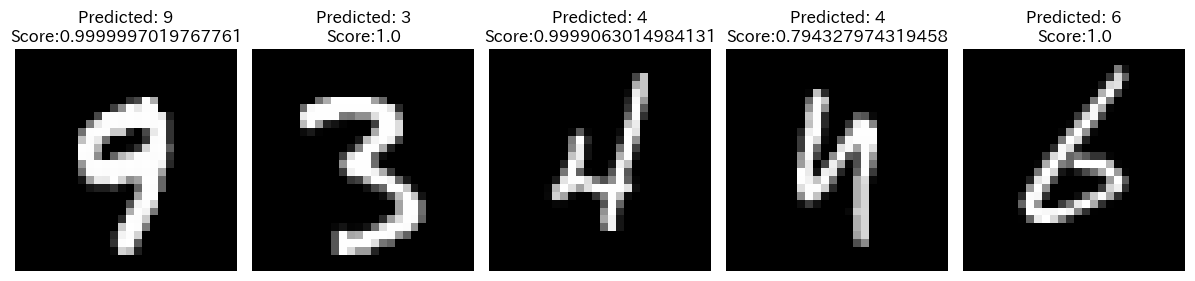
コード7は,画像とモデルによる判断の確認です。
Run code-7, then images and and predictions by the model show.
import numpy as np
import matplotlib.pyplot as plt

# テストセットからランダムに画像を抜き出す
# Select a random subset of images from the test set
num_images = 5
np.random.seed(seed=2)
random_indices = np.random.randint(0, len(x_test), num_images)
images = x_test[random_indices]
labels = y_test[random_indices]

# 選択した画像について予測する
# Make predictions on the selected images
predictions = model.predict(images)
predicted_labels = np.argmax(predictions, axis=1)

# 画像と予測されたラベルおよびスコアを表示する
# Display the images with their predicted labels and scores
fig, axes = plt.subplots(1, num_images, figsize=(12, 3))

for i in range(num_images):
    axes[i].imshow(images[i].reshape(28, 28), cmap="gray")
    axes[i].axis("off")
    axes[i].set_title(
        f"Predicted: {predicted_labels[i]}\nScore:{round(np.max(predictions[i]), 8)}"
        )

plt.tight_layout()
plt.show()
2.自然言語処理の機械学習/Machine Learning in Natural Language Processing
書籍では,AIの中でも最も注目を集めている,自然言語処理(NLP)について説明しています。
Natural Language Processing (NLP), the most popular type of AI at the moment, is explained in the English website.
12.2.9 感情分析を試してみよう/Let's Try Sentiment Analysis
下記コード8でライブラリをインポートします。
Import libraries with code-8.
# 必要なライブラリのインストール
# Installing necessary libraries
!pip install -q transformers
!pip install ipadic
!pip install fugashi
!pip install xformers
コード9で,Transformerに格納されている,クラスやモデル、パイプラインオブジェクトを呼び出せる状態にしておきます。
Running code-9 makes a class, a model, and a pipeline object stored in the Transformer ready to be called.
from transformers import AutoTokenizer,BertForSequenceClassification,pipeline
コード10ではエンコーディングをします。
Encoding is done by code-10.
# Tokenizerの読み込み
# Load the tokenizer
tokenizer=AutoTokenizer.from_pretrained("koheiduck/bert-japanese-finetuned-sentiment")

# モデルの読み込み
# Load the model
model = BertForSequenceClassification.from_pretrained("koheiduck/bert-japanese-finetuned-sentiment")
コード11で感情分析を実行します。
Sentiment Analysis is performed by running code-11.
print(pipeline("sentiment-analysis",model=model,tokenizer=tokenizer)
("私は幸福である。"))
print(pipeline("sentiment-analysis",model=model,tokenizer=tokenizer)
("I am happy."))