09最適化の考え方を用いた分析 / Analysis with the Concept of Optimization
【目次/TOC】
1. Excelにおける最適化/Optimization in Excel
9.1.1 ゴールシーク/Goal Seek

本ウェブページは『超入門 はじめてのAI・データサイエンス』第9章に関連する動画とコードを埋め込んでいるページです。
データアナリティクスのタスクには,統計的手法を用いる予測・分類や,反復計算で収束させる最適化などがあります。
今回は,Excelにおける最適化としてゴールシークを実習し,ソルバーを紹介します。
このセクションでは,ゴールシークで最適な解を探す操作を体感しましょう。
In this webpage, videos and codes corresponding to Session 09 of the English website are embedded.
Tasks in Data analytics include prediction and classification that use statistical methods, as well as optimization that converges through iterative calculations. In this session, we will practice Goal Seek and introduce Solver as optimization methods in Excel. In this section, you will experience finding the optimal solution with Goal Seek.
動画のシナリオは,次の通りです。 あるイベントでスイーツを販売するのに,スイーツ1個当たりの食材費(原価)が600円という想定です。販売価格から原価を引いた金額が粗利で,粗利が大きいほど当然販売価格が高くなり,予想される販売個数が少なくなります。 昨年度までのデータにより,その関係は,スイーツ販売個数=2000-1.1×粗利という線形近似(線形回帰モデル)で予測できることがわかっているとします。 このとき,総売上高を70万円にするには,その食品をいくつ作って,販売価格をいくらに設定すればよいか,その最適値を求めるというタスクです。 動画のデータは簡単に手入力で作成できます。
The scenario of the video is as follows. You would like to sell some sweets at an event and the cost of materials (cost price) for each sweet is 600 yen. The amount obtained by subtracting the cost from the selling price is the gross profit per unit, and the higher the gross profit, the higher the selling price and the lower the expected number of units sold. Suppose that the relationship can be predicted by a linear approximation (linear regression model), where the number of sweets sold = 2000 - 1.1 x gross profit, based on data up to the previous year. In this case, the task is to find the optimal value of how many sweets to make and how much to set the selling price in order to achieve total sales of 700,000 yen. It is very easy to manually input the data as shown in the video below.
リボンのデータ,What-If 分析,ゴールシークでゴールシークウィンドウを開き,数式入力セルに売上総利益の数式を入力したセル,その目標値を700,000にして, 変化させるセルに粗利のセルを入れて,ゴールシークをしています。 ゴールシークはExcelが反復計算をしてゴールに到達する様子が見て取れる,最適化の原型のような機能です。
To open the Goal Seek window, click Data > What-If Analysis > Goal Seek... In Set cell enter the cell with gross profit formulas, in To value enter 700,000, and in By changing cell enter the cell for the gross profit per unit. Goal Seek is a prototypical method of optimization that allows you to see and feel how Excel iteratively calculates to reach a goal.
9.1.2 ソルバー/Solver
ソルバーは, 昨年度までの経験ではPCが固まってしまう人が複数名発生したので,動画を視聴するにとどめましょう。Excelでソルバーを利用するにはアドインが必要です。 このセクションでは,上のゴールシークの例よりもやや複雑な例について,ごく短い動画で説明します。ソルバーでは,目的の設定と,そのために最適化するセル範囲の他に,「制約条件」を入れることが出来ることについて理解をしてください。
You can just watch the video, as I have seen Solver has caused several people to freeze their PCs. To use Solver in Excel, you need to do add-in. In this section, a very short video is provided to illustrate a slightly more complex example than the Goal Seek above. You should understand that solvers can include "constraints" in addition to setting the goal and the range of cells to be optimized for it.
ソルバーによって解決すべきタスクはつぎのようなシナリオです。みなさんは17人グループの旅行の幹事でレンタカーを借りたいとします。そしてレンタカー屋のホームページから 得られた情報はB列とC列の2列,それぞれの車種が何人乗りか,そして時間当たりの金額だとします。 17人でレンタカーを借りて旅行をするのに,AからJまである車種のどれを何台借りると金額が安く済むか?という問題を解決するというタスクです。
The following scenario is the task to be solved by Solver here. You are the organizer of a trip for a group of 17 people and you want to rent a car. The information obtained from the website of the car rental agency is in Columns B and C, the capacity of passengers and the price per hour for each type of car. The task is to solve the problem of how many of each type of car from A to J should be rented for a trip for 17 people at the lowest price.
レンタカー屋のウェブサイトから得た情報は2列(p.121 表9.2の列B & E)ですが,動画のソルバー実施に向けて,(1)の準備作業が必要です。
(1) ここは動画にはありませんが,借りる台数,その車種に乗車する人員数,金額,の3列は,全体の支払い金額を計算するためにみなさんが追加したものとします。
乗車人員数には,何人乗り×台数の数式を入力します。金額にも、時間当たり金額×台数の数式を入力しました。
乗車人員数の列と金額の列には,合計の関数を入力しました。
17人なので,台数はとりあえず10人乗りを1台と7人乗りを1台と手入力してみると,支払金額は時間当たり10,100円となりました。もっと安くすることはできるでしょうか?
ここからが動画で,ソルバーの登場です。
The information obtained from the car rental agency's website is in the two columns B and E, but preparatory work is needed for (1) to implement the solver for the video.
(1) This is not in the video, but the three columns, the "number of cars" rented, the "number of passengers" in that car type, and "total price", should be added to calculate the total amount paid.
For the number of passengers, I enter the formula for the number passengers x the number of cars. For the "total price", I also enter the formula for the "price" per hour x "number of cars".
In the columns for the number of passengers and the column for the total price, I enter the SUM functions.
Since there are 17 passengers, I entered one 10-passenger car and one 7-passenger car tentatively, and the amount to be paid was 10,100 yen per hour. Is it possible to make it cheaper? .
This is where Solver comes in.
ソルバーは,与えられた条件での最適解を返してくれます。この場合,緑のセルで17人以上が乗車可能となることが条件で,黄色のセルの合計金額を最小にするための最適解を,赤の範囲で調整して求めてくれます。
Solver returns the optimal solution under the given conditions. In this case, it finds the optimal solution to minimize the total amount of money in the yellow cells by adjusting the red range, provided that more than 17 people can be accommodated in the green cells.
動画ではつぎの(2)~(6)を実施して最適解を得ています。
(2) リボンのデータから,ソルバーをクリック。「目的セルの設定」で,黄色のセルを設定します。
この金額を一番安くしたいので,「目標値」を「最小値」にします。
(3) 「変数セルの変更」で,最適解を求めたい赤い範囲を設定します。
(4) 「制約条件の対象」の欄の中をクリックして「追加」ボタンをクリック。
セル参照を赤い範囲,それを整数(int)に指定して,追加ボタン。
In the video, the following (2) through (6) are performed to obtain the optimal solution.
(2) From the ribbon, click on Solver. In the "Set Objective" section, set the yellow cell.
Choose the "Min" radio button, since we want this amount to be the lowest.
(3) In "By Changing Variable Cells", set the red range where you want to find the best solution.
(4) Click inside the "Subject to the Constraints" and click the "Add" button.
Enter the red range into Cell Reference and in Constraint make it as an integer (int), and click the Add button.
(5) 「追加」ボタンで条件の追加。セル参照を緑のセル,それを17以上に指定して,「OK」ボタン。そして,「解決」ボタン。
(6) ソルバーの結果が出たら「OK」。
最適解が返されて,支払金額は7,500円になりました。Cを3台,AとBを1台ずつ借りると,もっとも安く済むことがわかりました。これでソルバーを使って問題を解決することができました。
(5) Add a condition with the "Add" button. Enter the green cell as the cell reference and make it as 17 or more, and click "OK" button. Then, "Solve" button.
(6) When you get the result of the solver, click "OK".
The optimal solution is returned, and the amount to be paid is 7,500 yen, which turns out to be the cheapest if we rent 3 Type-C cars, 1 Type-A car and 1 Type-B car. We could use Solver to solve the problem.
2.Pythonによる最適化/Optimization with Python
9.2.1 ソルバー/Solver
ここでは,PuLPライブラリを使って,上述のソルバー問題をPythonを用いて実行する方法を紹介します。コード1で必要なPuLPライブラリをインストールして読み込みます。
We will show you how to solve the same solver task as described above with Python, using the PuLP library here. Code-1 will install and import the PuLP library.
!pip install pulp
import pulp
下記コード2はモデルを作成しています。#車種以下で,上のExcelソルバーと同じ条件を与えています。
Code-2 below creates a model. The lines following "# Car models" give the same conditions as the Excel solver above.
#モデル
model = pulp.LpProblem('rent',sense = pulp.LpMinimize)
# 車種 /  Car models
car = ["a", "b", "c", "d", "e", "f", "g", "h", "i", "j"]
# 人乗り /  Capacities
capacity = [2, 3, 4, 4, 6, 7, 8, 8, 8, 10]
# 金額 / Prices
price = [1200, 1500, 1600, 2400, 3000, 3300, 3800, 4600, 5000, 6800]
コード3は、最適化したい(各車種からレンタルする)「台数」をxsとして変数を定義します。コード4でモデルを完成させます。コード5でソルバーを起動すれば,上のExcelのソルバーで得たものと同じ解が返ることが確認できます。
Code-3 defines the variable "xs", the number of cars to be rented for each model, that you want to optimizethe. Code-4 completes the model. Starting the solver with code-5 will result in returning the same solution as the one obtained in the Excel solver above.
# 変数の定義 / Define the variable
xs = [pulp.LpVariable("{}".format(x),cat="Integer",lowBound=0) for x in car]
# 目的関数 / Objective (function)
model += pulp.lpDot(price,xs)
# 制約条件 / Conditional constrains
model += pulp.lpDot(capacity,xs) >= 17

print(model)
status = model.solve(pulp.PULP_CBC_CMD(msg=0))
print("Status",pulp.LpStatus[status])
print([x.value() for x in xs])
print(model.objective.value())
9.2.2 主成分分析の考え方/Concept of Principal Component Analysis
「最適化」そのものからは逸れますが,その考え方の実用的な応用例として,主成分分析による次元削減をPythonで実行してみましょう。いくつもの特徴量があるところから何かを見分けるときに、特徴量の数すべてのn次元の中から見分けようとするよりも、個体の違いを見分けやすい次元に削減したい場合があります。個体の違いを見分けやすくするために、分散を最大化する軸に次元を削減するのが主成分分析です。
While we digress from optimization here, let's experience with Python dimensionality reduction by Principal Component Analysis as a practical application of the idea of maximization. When distinguishing something from a number of features, rather than trying to distinguish among all n dimensions of the number of features, we may want to reduce the dimensionality to some distinctive dimensions that makes it easier to distinguish individual differences. To make it easier to distinguish differences between individuals, Principal Component Analysis reduces the dimensions to the axes that maximizes the variance.
たとえば書籍 p.114 図8.2の散布図では,ペンギンの種を見分けることは困難です。この散布図で3つのペンギンの種がどのような散らばりを見せていたのか,下記コード6で種ごとに色を付けて見てみましょう。書籍 p.125 の図9.1を表示します。
With the scatterplot of Figure 8.2 in Session 08, for example, it is difficult to distinguish the penguin species. Let's color each species and see how the three penguin species are scattered in the same scatterplot with code-6 below. Figure 9.1 of Session 09 will be displayed.
import seaborn as sns
import matplotlib.pyplot as plt
import numpy as np
df = sns.load_dataset('penguins')

X = df['flipper_length_mm'].values
Y = df['body_mass_g'].values

sns.set_style("white")
color = ["#87CEEB", "#2E8B57", "#F4A460"]
sns.set_palette(color)
sns.scatterplot(data=df, x=X, y=Y, hue="species")
plt.xlabel("flipper length [mm]")
plt.ylabel("body mass [g]")
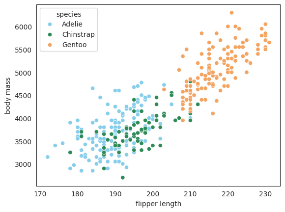
Figure 9.1 Scatterplot of Flipper Length and Body Mass Colored by Species
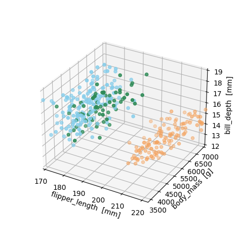
別の軸を加えて3次元にすると,種がもっと見分けやすくなります。それが下記のコード7で,書籍 p.125 の図9.2を表示します。
If we add another axis and make it 3 dimensional, the species become more discernible. Figure 9.2 of Session 09 is what code-7 below will display.
fig = plt.figure(figsize=(8,6))
ax = fig.add_subplot(projection="3d")

x = df["flipper_length_mm"].values
y = df["body_mass_g"].values
z = df["bill_depth_mm"].values

axes = plt.axes(projection="3d")

colors = np.where(df["species"]=="Adelie","#87CEEB","-")
colors[df["species"]=="Chinstrap"] = "#2E8B57"
colors[df["species"]=="Gentoo"] = "#F4A460"

ax.set_xlabel("flipper_length [mm]")
ax.set_ylabel('body_mass [g]')
ax.set_zlabel('bill_depth [mm]')

axes.scatter3D(x, y, z, c=colors)
ax.set_box_aspect(aspect=None, zoom=0.8)
いよいよ主成分分析に向けた準備です。主成分分析を行うためには欠損値を処理しておかなければならないので、コード8で欠損値を削除し,その結果を確認しています。欠損値がなくなっているとともに,ペンギンの量的データの特徴量が4つあったことも再確認できたでしょうか。主成分分析では,この4次元を2次元に削減します。コード9では,df3の3列目から6列目までの量的データのスケールを統一するために,標準化(平均を引いて標準偏差で割ること)したデータフレームdf4を作成します。
code-8 Let us prepare data for Principal Component Analysis. Since missing values must be deleted in order to perform a Principal Component Analysis, let's remove the missing values with code-8 and check if the missing values have been eliminated. Also reconfirm that there are four features of the quantitative data of the penguins. With a Principal Component Analysis, we will reduce these four dimensions to two. Code-9 standardizes (subtracting the mean and divided by the standard deviation) the quantitative data in the columns 3 to 6 of df3 in order to put them onto the same scale, and name the data frame df4.
df3 = df.dropna()
df3.head()
df4 = df3.iloc[:,2:6].apply(lambda x:(x-x.mean())/x.std(), axis=0)
df4.head()
下記コード10で主成分分析を実行し,各個体の成分得点をfeatureに格納します。
Runnning code-10 will perform the Principal Component Analysis and assign principal component scores of the penguins into "feature".
import sklearn
from sklearn.decomposition import PCA
pca = PCA(n_components=2)
pca.fit(df4)
feature = pca.transform(df4)
下記コード11では成分得点をデータフレームにしたものをdf5にしています。すでにpandasライブラリが読み込まれていることが想定されています。
Code-11 below creates df5, a data frame consisting of the principal component scores. The code supposes that pandas is already imported.
df5 = pd.DataFrame(feature, columns=["PC{}".format(x+1) for x in range(2)])
df5.head()
下記コード12がつくるのは,2次元に削減した散布図(書籍 p.127 図9.4)です。同じ2次元でも図9.1に比べてどれほど種が見分けやすくなっているか,いわば答え合わせのために色付けをしています。色付けのために,種の列の残っているdf3を呼び出して各ペンギン種に色を与えています。
Code-12 below creates a scatterplot in the reduced two dimensions (Figure 9.4 of Session 09). It is colored to see that species become more easily discernible than Figure 9.1 while both plots being two-dimensional. For coloring, df3, which retains the species column, is used to give each penguin species a color.
colors = np.where(df3["species"]=="Adelie", "#87CEEB", "-")
colors[df3["species"]=="Chinstrap"] = "#2E8B57"
colors[df3["species"]=="Gentoo"] = "#F4A460"

plt.figure(figsize=(6,6))
plt.scatter(feature[:,0], feature[:,1], alpha=0.8, c=colors)
plt.grid()
plt.xlabel("PC1")
plt.ylabel("PC2")
plt.show()
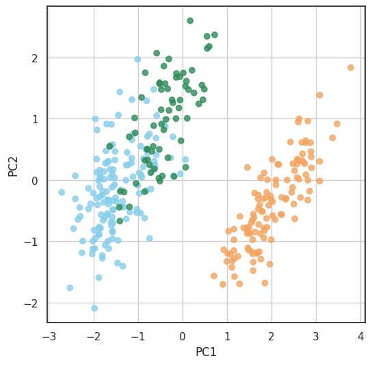
この例では特にジェンツー種が見分けやすくなっていますが,同じような手法で,病変した組織や,人間には知られていなかった種類の違いを見分けることに役立てることができることが想像できたでしょうか。Pythonコードを書いていくことを学ぶことはそれを目的としている別科目に譲るとして,ここでは,分散を最大にする主成分分析と,それが可能にする次元削減の可能性を理解してもらえればと思います。
In this example, the gentoo is particularly easy to distinguish, but imagine how this technique may apply to discoveries of disease, previously unknown species, and so forth. I leave the details of how to write Python code to other courses designed for that purpose, and hope that here you understood the potentials of dimensionality reduction such as Principal Component Analysis that maximizes variances.