10統計的推定と仮説検定 / Statistical Inference and Hypothesis Testing (1)
【目次/TOC】
1. 仮説にかんする用語/Terms Related to Hypotheses

本ウェブページは『超入門 はじめてのAI・データサイエンス』第10章の10.1, 10.2に対応したコードを埋め込んでいます。ここでは2つの変数の関係 (1),xyの両方または片方が質的データである場合について,統計の基礎的な部分を抜粋してお伝えします。
This webpage corresponds to 10.1 and 10.2 of Session 10 of the English website. Here we show some examples of basic statistics for the relationship between two variables (1) when both or one of x and y are qualitative data.
変数の関係は一般に変数xyの関係として表されます。
x:仮説において原因となる方の変数で,独立変数または説明変数と呼ばれる
y:仮説において結果となる方の変数で,独立変数が与えられたときにその値に従属して値が動くので従属変数または説明変数が説明しようとする目的であるので目的変数と呼ばれる
xyが2つとも質的変数の場合がクロス集計表,xが質的変数,yが量的変数の場合が平均の比較になることについて,下の短い動画を参考にしてください。
In expressing relationships between variables:
x: the cause in the hypothesis, called the independent variable or explanatory variable
y: the outcome in the hypothesis, called the dependent variable because its values are dependent on some given independent variables, or response variable.
Please refer to the short video below which shows that when xy is both qualitative variables we use cross tabulation, and when x is a qualitative variable and y is a quantitative variable, we compare means.
Video with English subtitles
2.質的変数を含む変数の関係 / Relationships with Qualitative Variables
10.2.1 Excel で考えるカイ二乗検定 / Understanding Χ2 Test in Excel
\(\chi^2\)検定を実施するときには,Excelよりも統計に便利なツールを使うことが多いので,操作を覚えることは重要ではありません。デモンストレーション用の動画を視聴して\(\chi^2\)検定の意味を理解してください。データは第2章と第3章(3.1.1)で作成したもの(具体的には,ダウンロードしたCopyFromHere01.xlsxにCopyFromHere03.xlsxを合体させたもの)を用います。Excelのクロス集計表の作り方はピボットテーブル(第3章)も参考にしてください。
When conducting a \(\chi^2\) test, we often use more convenient tools for statistics than Excel, so it is not important to learn the Excel operations. Watch the demonstration video to understand the meaning of \(\chi^2\) test. We use the data we created in Chapters 2 and 3 (3.1.1) (specifically, the downloaded CopyFromHere01.xlsx combined with CopyFromHere03.xlsx). See Pivot Table (Session 03) for how to create a cross-tabulation table in Excel for your reference.
レンタカーとしてレンタルされる車種は都市によって異なるか?という問いがあったとします。各都市におけるレンタカーが数ある中で(母集団),自社で把握しているレンタカーのデータをサンプル(標本)だと考えると,これは統計的推測の問題です。たとえ都市によってレンタル車種が異ならないとしても,取得したデータ上ではレンタル車種の割合がぴったり一致するなどということは珍しく,大抵割合の異なるデータになります。データに見られる差はサンプルの抽出上たまたまという範囲内なのか,それとも母集団で都市によって割合が異なるために生じる差なのかについて統計的推定を行い,理論的標本分布を用いて,「レンタルされる車種は都市によって異ならない」という帰無仮説が棄却されるかどうかをを検定します。この場合,支店も車種も質的変数なので,クロス集計表を作ります。動画はクロス集計表を作るところからはじまります。 後にお話しする理由によって、今回は車種はA~Cだけに絞ったクロス集計表を作ります。
Does the type of car rented vary from city to city? Since cars rented in each city is the population, and the data we have on car rentals is a sample, this task involves statistical inference. Data usually show different percentages. Even if data are taken from the population where rental car types do not vary from city to city, it is highly unlikely that each car type has the exact same percentage in a sample. We perform statistical inference of whether the differences in the data are just a matter of chance caused by the sampling or whether they are due to differences in the population. The null hypothesis is that "car types rented are not different by city". Using theoretical sampling distribution, we test whether the null hypothesis can be rejected. In this case, since both branch and car type are qualitative variables, we create a crosstabulation table and the video begins from here. For reasons we will discuss later, we will create a crosstabulation table with only car types A to C.
つぎに,xyに関連がなかった場合に期待される表,つまり帰無仮説が正しい場合の表を作ります。それを,期待度数表と言います。
各セルの期待度数は,\[i行目j列目のセルの期待度数=n×\frac{行iの計}{n}×\frac{列jの計}{n}\] となります。ただし\(n\)は全個数です。
ハット(^)の記号は,期待値という意味
\(f\)はfrequency,度数
\(i\)は\(i\)行目,\(j\)は\(j\)列目
とすると、\(\hat{f_{ij}}\) つまり\(i\)行目\(j\)列目のセルの期待度数は次の数式で表すことができます。
\[\hat{f_{ij}}=\frac{(f_i.)(f_.j)}{n}\]
Next, create the table expected when xy were not related, that is, if the null hypothesis is true. It is called expected frequency table. The expected frequency of each cell is: \[expected \, frequency \, of \, row \, i, \, column \, j = n×\frac{total \, of \, row \, i}{n}×\frac{total \, of column \, j}{n}\] n is the total number of cells. The hat (^) symbol indicates expected value, f is frequency, i is row i, and j is column j. The expected frequency of the cell in row i, column j \(\hat{f_{ij}}\) can be expressed by the following formula: \[\hat{f_{ij}}=\frac{(f_i.)(f_.j)}{n}\]
それでは観測度数表の観測値は,期待度数表からどの程度離れているでしょうか?
各セルの差を出して足してしまうとプラス・マイナスが相殺されてゼロになってしまうので,差を二乗します。それを期待値で割って大きさの調整をしたものを,表のすべてのセルについて合計します。
\[\chi^2=\displaystyle\sum_{i=1}^{R} \sum_{j=1}^{C} \frac{(\hat{f}_{ij}-f_{ij})^2}{\hat{f}_{ij}}\]
ただし:
∑は総計
Rは行(row)の数
Cは列(column)の数
この値をカイ二乗値(\(\chi^2\))と呼び,この値が大きいほど期待度数から観測度数がずれていることを示します。
How far are the observed values from the expected frequency?
If we take the difference of each cell and add them together, the positive and negative values will cancel each other out and become zero, so we square the difference. Then divide it by the expected value to adjust for size, and sum it for all cells in the table.
\[\chi^2=\displaystyle\sum_{i=1}^{R} \sum_{j=1}^{C} \frac{(\hat{f}_{ij}-f_{ij})^2}{\hat{f}_{ij}}\]
Where:
∑ is total
R is the number of rows
C is the number of columns
This value is called chi-square, and the larger this value is, the more the observed frequencies deviate from the expected frequencies.
Video with English subtitles
Windows/English
Mac/日本語
10.2.2 仮説検証の考え方/Idea behind Hypothesis Testing
しかし,\(\chi^2\)がどんなに大きい値だからと言って,帰無仮説が正しい場合でも,その値が絶対にありえないとは言えません。
そこで,ある程度あり得ないと言える場合には帰無仮説を棄却して,xyに関係があるとする対立仮説を採択してよいと考えるのです。
これが統計的検定の考え方です。
帰無仮説を棄却する水準は分析者が設定し,それを有意水準と言います。
有意水準αは0.05や0.01などキリの良い値に定めます。
帰無仮説が正しい場合に,自分の標本から得た検定統計量の値よりも起こりにくい値が生起する確率であるp値(有意確率)を比べて,\(p<\alpha\)の場合に帰無仮説を棄却します。
この\(p\)値偏重型の考え方には色々議論もあるのですが,まずはこの伝統的な考え方を理解することが肝要です。
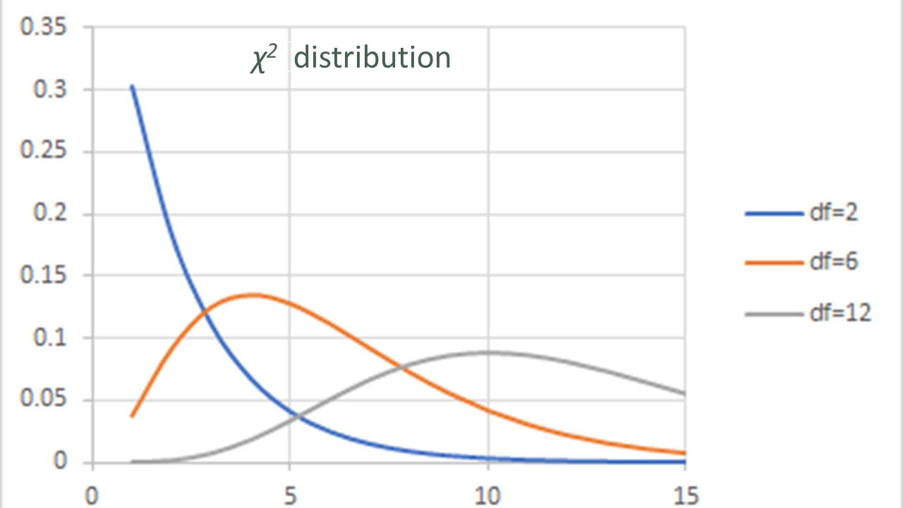
\(\chi^2\)の確率分布は自由度 df(degrees of freedom)により形が決まっています。
クロス集計表のdf: (R-1)×(C-1)
No matter how large \(\chi^2\) is, however, we cannot say that the value is absolutely improbable even when the null hypothesis is true.
Therefore, if the null hypothesis can be said to be implausible to a certain extent, we reject the null hypothesis and adopt the alternative hypothesis that says there is a relationship between x and y.
That's how statistical testing is done.
Significance level, the level at which the null hypothesis is rejected, is set by the analyst.
The significance level α is set to a close value such as 0.05 or 0.01.
We compare the p value (significance probability) with α. The p value is the probability of the test statistic from our sample and values less likely to occur than than that value when the null hypothesis is true,. We reject the null hypothesis if p < α.
There is a lot of discussion about this p-centered approach, but it is important to understand this traditional approach in any case.
The probability distribution of chi-squared depends on degrees of freedom df.
df in cross tabulation tables: (R-1)×(C-1)
そして動画では,表計算で\(\chi^2\)値を計算し,そこから
CHISQ.DIST.RT関数を使ってカイ二乗分布でその\(\chi^2\)値より大きな値をとる確率つまり右片側面積(right tail)を求めるとともに、
CHISQ.TEST関数を使って\(\chi^2\)検定を行って求めた
p値と一致することを見せています。
\(p≧\alpha\)のときには,帰無仮説は棄却できません。報告書にはたとえば次のように書きます。
「支店と車種のクロス集計表で\(\chi^2\)検定を行ったところ,\(\chi^2\)=13.89,df=12,p=0.308であった。
よって,支店と車種A~Cがレンタルされる頻度には統計的に有意な関係があるとはいえない。」
In the video, Chika-chan calculated the chi-squared in a spreadsheet, and from there used the RT function to find the the right tail probability, that is, the probability of taking a value greater than its chi-squared in the chi-squared distribution.
Then Chika-chan used CHISQ.TEST function to obtain the p value to show the results are consistent.
When p ≧ α, the null hypothesis cannot be rejected. The results are reported as, for example,
"The relationship is not statistically significant by a chi-squared test, \(\chi^2\) = 13.89, df = 12, and p=0.308. Therefore, there is no statistically significant relationship between cities and the types of the rented cars (A to C)."
このように,検定というのは操作自体は簡単で,統計ソフト等を使えばもっと簡単です。だから分析者が知っておかなければならないのはむしろ分析の意味と,どういうときに使うか,そして使ってはいけないか,です。 \(\chi^2\)検定も使わない方が良い状況というのがあって,期待度数が5未満のセルが20%以上か、最小期待度数が1未満のセルがあるときは\(\chi^2\)検定は行わないことになっています。 車種D以降を分析に入れてしまうとこの条件に引っかかってしまうために,今回車種A~Cのみを選んだのでした。
As you can see, conducting a test itself is easy, and even easier if you use some statistical software. Therefore, what you need to know is the meaning of the analysis, when to use it, and when not to use it. There are some situations in which we should not use the chi-square test: when there are more than 20% of cells with an expected frequency of less than 5 or when there are cells with a minimum expected frequency of less than 1, we should not use the chi-square test. I included only car models A through C in the analysis because including car models D and beyond would violate the criteria.
10.2.3 分散,標準偏差,Z得点(標準化)/Variance, Standard Deviation,and Z Score (standardization)
ここから量的変数の統計的推定の話になるので,量的データの分布に関して3つの分布に分けて考えます。
第1の分布: 母集団の分布
第2の分布: 標本の値の分布
第3の分布: 統計量の確率分布
第1の分布は,分析者が知りたい分布です。分析者が分析によって知りたい母集団の特徴を示す母数をパラメータと言います。母集団の全数を調べる全数調査は叶わないことが多いので,標本調査をして,母集団から標本として抽出したデータからパラメータを推定します。それが統計的推定です。分析者が観察することができるのは,抽出したひとつの標本のデータの値であり,その値の分布が第2の分布です。第3の分布は,母集団からありとあらゆる組み合わせで大きさNの標本を抽出してその1つ1つの標本から統計量を算出したとして,その統計量の理論的分布です。標本ひとつひとつがデータとなるので標本分布です。統計的検定は標本分布を用いて行わることが多く,上記の\(\chi^2\)検定で利用した\(\chi^2\)分布は,\(\chi^2\)値という統計量の理論的な確率分布なので,第3の確率分布のひとつです。
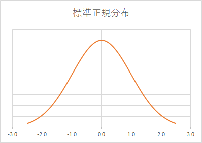
第3の分布でよく使われる,正規分布,t分布など左右対称の釣り鐘型の分布の特徴は,平均値と標準偏差という2つの特徴で把握します。
Since we are now talking about statistical inference of the quantitative variable, we conceptualize what I call three types of distributions of quantitative data.
The first-type distribution: distribution of values in the population
The second-type distribution: distribution of values in a sample
The third-type distribution: probability distribution of a statistic
The first distribution is the distribution that the analyst wants to know about. Numbers that represent population characteristics that the analyst wants to know by conducting analyses is called parameter. Since it is often not possible to conduct a complete enumeration of the entire population, a sample survey is conducted and the parameters are estimated from data extracted as a sample from the population. That is statistical inference. What the analyst can actually observe is the values of the data in a single extracted sample, and the distribution of those values is the second distribution. The third distribution is the theoretical distribution of a statistic, assuming that every possible sample of size n is extracted from the population and that a statistic is calculated from each sample. It is called sampling distribution because such statistic from each sample becomes data. Statistical tests are often conducted using sampling distributions, and the chi-squared distribution used in the chi-square test above is one of the third-type distributions because it is the theoretical probability distribution of the statistic of chi-squared.
The characteristics of symmetrical bell-shaped distributions such as the normal distribution and t-distribution, which are frequently-used third-type distributions, can be summarized with mean and standard deviation.
それではまず(第2の分布のうち推定も何もしない)全数調査のデータで,みなさんが高校で学んだ,量的変数の値の変動(ちらばり)の大きさを表す2つの記述統計量,分散(variance)と標準偏差(standard deviation)のおさらいから始めましょう。上司からこんな質問を受けたとします。「今年は若い人から高齢者までうちのサービスを利用してくれて,去年より年齢のばらつきが大きくなった気がするんだけど,どうかな?」 このタスクを言い換えると,第2の分布の値の変動の大きさを統計量で把握して昨年度の値と比較するタスクです。考え方をExcelで体感しましょう。 年齢の高い人は平均値から上に離れている,年齢の低い人は平均から下に離れていて,そういう平均との差を偏差といいます。 ばらつきが大きいということは、偏差の絶対値が全体的に大きいということです。 標本分散s2とは、偏差平方和をnで割ったものです。(注:第1の分布の分散を推定したい場合の不偏分散はnではなくて自由度n-1で割ります。) \[s^2=\frac{\sum (y_i-\hat{y})^2}{n}\] 標準偏差\(s\)とは分散の平方根です。 \[s=\sqrt{s^2}\]
Let's start with reviewing the two descriptive statistics that you all should have learned in high school, variance and standard deviation, which express the degree of variation of the values of a quantitative variable, using our data taken as complete enumeration (as a second-type distribution with no need for estimation). Suppose your boss asks you a question like this "This year we have had both young and old people using our services, and I think the age variance has increased since last year. To rephrase our task, we need to summerize the magnitude of the variation in statistics and compare the value with that from the last year. Let's experience the concept in Excel. The older people have ages above the mean, the younger people below the mean, and the differences from the mean is called deviation. A large variation means that absolute values of deviations are large overall. The variance based on the entire population s2 is the sum of squared deviations divided by n. (Note: If you estimate the variance of the population from a sample, you should use unbiased variance where the sum of squared deviations is divided by degrees of freedom n-1 , not n.) \[s^2=\frac{\sum (y_i-\hat{y})^2}{n}\] The standard deviation \(s\) is the square root of variance. \[s=\sqrt{s^2}\]
今年の年齢の全般的なばらつき度合い,つまり偏差の平均的な値を求めようとすると上記の式になることを実習で体感してみましょう。 下の動画を観ながら「Input Data」のワークシートでの実習で手を動かして,高校時代に学んだ変動の統計量を思い出してください。 まずは,Age(動画では「年齢」)の列を用いて,隣の列を「AVERAGE」と名付け,複合(もしくは絶対)参照のAVERAGE関数で平均年齢をオートフィルします。
Experience through the practice that if you would like to have the general degree of variation, that is, the average deviation of age in this year's data, you'll come up with the formula above. Watching the video with the hands-on practice on the "Input Data" worksheet may remind you of the statistics of variance and standard deviation you learned in high school. First, find the column "Age", name the adjacent column "Average" and use AVERAGE function and mixed (or absolute) reference to autofill the average age.
更にとなりの列をD(偏差)として,個々のデータの,平均との差を求めます。この平均との差が偏差です。 列の一番上のセルに偏差が入るように入力したら,下までオートフィルまたはフィルハンドルをドラッグしてコピーすれば,自然に相対参照になるので,偏差の列の完成です。 この偏差で全体の変動の大きさを見たいのですが,偏差を単に合計するとプラスとマイナスで相殺されてしまいます。
Name the next column D (for deviation), and enter the difference between the individual data and the mean. This difference from the mean is the deviation. Enter a deviation in the top cell of the column, then copy the data by autofill or dragging the fill handle to the bottom, which will result in a relative reference, thus completing the Deviation column. We want to see the total magnitude of the variation from the deviations, but if we simply sum the deviations, the pluses and minuses will cancel each other out.
そこで二乗して正の値にします。隣の列を「\(D^2\)」(偏差平方)とし,偏差を二乗した偏差平方を入力します。Excelではべき乗は 演算子^[キャレット]を使うのでしたよね。一番上のセルに偏差平方が入ったら,同列を同様にフィルします。この偏差平方の平均を出したいので,総和してNで割りましょう。 偏差平方を合計した偏差平方和を任意のセルにオートSUMで入力しましょう。平均を出すときみたいに偏差平方和をN=200で割った値を算出すれば,分散 (variance) を計算したことになります。 別のセルにはVAR.Pで,標本分散の関数を入れてみましょう。 図のように関数の戻り値と,自分で計算した分散の値は一致するはずです。
So, square deviations to make them positive. The next column is D2 and enter squared deviation using ^ [caret] operator for exponentiation in Excel. Once you entered a squared deviation in the top cell, fill in the same column in the same way. We want to get the average of the sume of squared deviations, so we will sum them up and divide by N. Enter the sum of squared deviations in any cell using AutoSUM. If you divide the sum of squared deviations by N=200, the returned valued is variance. In another cell, put VAR.P, variance based on the entire population. The returned value of the funccion must match the variance you calculated.
VAR.PのPは母集団 (population)のPで,全数データ(データ自体が母集団)のときの分散はこれを選びます。
分散はばらつきが大きいほど大きな値になりますが,計算過程で二乗しているので「平均からの標準的な偏差」というには大きすぎる値になっています。
そこで平均からの標準的な偏差となるような数値を求めるため,分散にルートをかけて元の大きさに戻します。
この値が,標準偏差 (standard deviation) で,平均からの標準的な偏差を示す統計量です。
自分で計算した標準偏差と関数の標準偏差の値を比べてみましょう。任意のセルにSTDEV.Pという標準偏差の関数を使って標準偏差を表示させて,自分で計算した標準偏差と一致するのを確認してください。
P after the dot in VAR.P is P of population, and this function is used to calculate the variance for complete enumeration data (the data itself is the population).
The larger the variance, the larger the scatter of the values, but since it is squared in the calculation process, its value is too large for a measure of standard deviation from the mean.
So, the variance is square-rooted to adjust its size in order to obtain standard deviation.
Please compare the value of the standard deviation you calculated yourself with the returned value of the function STDEV.P. In any cells, display the standard deviation using the function and the standard deviation you calculated yourself. See for yourself that they match.
ところで,Excelの統計関数には,VAR.S関数と STDEV.S関数という選択肢もあります。このSは標本(sample)のSです。 データが母集団(第1の分布)から抽出した標本で,知りたいのが標本(第2の分布)自体の分散・標準偏差ではなく,抽出元の母集団の分散・標準偏差の推定値(第1の分布のパラメータ)であるときには,こちらを選びます。統計の主目的のひとつはパラメータを推定することと言っても過言ではありません。サンプルから知りたいのは第1の分布を特徴づける値である,母平均\(\mu\)と母分散\(\sigma^2\)および母標準偏差\(\sigma\)というパラメータです。 その場合はVAR.S関数の不偏分散,その平方根であるSTDEV.S関数を使います。ふつう使われるのはこちらなので,STDEVはSTDEV.Sと同じです。実習では,D2(偏差平方)の隣の列をSTDEVとし,複合参照(もしくは絶対参照)でSTDEV.Sをオートフィルしておきましょう。
By the way, Excel also has the VAR.S function and STDEV.S function. The S after the dot is the S of sample. When the data are a sample extracted from a population (the first-type distribution) and what you want is not to know the variance/standard deviation of the sample (the second-type distribution) but to estimate the variance/standard deviation of the original population (parameters in the first-type distribution), you should choose this option. It is safe to say that one of the main purposes of statistics is to estimate parameters. What we want to know from a sample are the values that characterize the first distribution: the parameters of the population mean \(\mu_Y\) , the population variance \(\sigma^2\) and the population standard deviation \(\sigma\). What we usually use is unbiased variance, VAR.S, and its square root, the STDEV.S, so STDEV is the same as STDEV. S. In the practice name the column next to D2 as STDEV and autofill them with STDEV.S.
次のタスクです。引き続き上司と雑談しています。上司の甥っ子は25歳の高橋蓮くん。このあいだ,この会社のサービスを利用したそうです。 「甥っ子の蓮は,うちのサービス利用者の中でどれぐらい若い方なのかなぁ。」と上司は首をひねっています。みなさんなら何と答えますか?
Next task. Suppose you are still chatting with your boss. Your boss's nephew is 25-year-old Ren Takahashi, who recently used the services of the company. Your boss is wondering: "How young my nephew Ren is among our service users?" Can you respond to this question?
ある顧客が分布の中でどの位置にいるのか,異なる分布の中での位置を比べるには,どんな統計量を使いますか? 異なる分布でも,平均が0,標準偏差が1になるように調整すれば,各データの全体の中での位置を比べることができますね。 これを標準(化)得点(z)といいます。「値を標準化してください」といわれたら、標準得点zに変換することを意味します。 zとは,平均が0,標準偏差が1になるように標準化したものですが、その平均を50,標準偏差を10に変換したものが,偏差値です。 逆にいうと,偏差値の50点を0に,10点の間隔を1にしたものがzだと考えれば,イメージが容易ですね。みなさんも,画像を参考にして年齢のZ得点を平均と標準偏差から計算してみてください。 その自分で計算したZ得点を,関数のSTANDARDIZEで標準化した値と比較します。両者は一致しましたか?
What statistic would you use to compare positions of given customers in different distributions? You can compare the position of each data within different distributions by adjusting them by making the mean 0 and one standard deviation 1. This is called standard score (z). When you are asked to "standardize values," this means to convert them to standard scores z. Just as z is standardized so that the mean is 0 and the standard deviation is 1, hensachi in Japanese is standardized so that the mean is 50 and the standard deviation is 10. If you are familiar with Japanese hensachi it is easy to conceptualize z by converting the score 50 to 0 and the interval of 10 to 1. Please refer to the image below and try calculating the z scores of Age using the mean and the standard deviation. Compare the z scores you calculated with the returned values of the function STANDARDIZE. Do they match?
Video with English subtitles
Windows/English
Mac/日本語
10.2.4 中心極限定理 (CLT)/Central Limit Theory (CLT)
中心極点定理と信頼区間について読んで理解しましょう。中心極点定理によると,ありとあらゆる\(\overline{y}\)の分布である第3の分布は一定の特徴を持った正規分布になります。信頼区間はt分布等を使って、\(\mu_y\)(変数yの母平均)などの母集団のパラメータを区間推定をすることができるものです。
Read and understand the Central Limit Theorem and confidence intervals with the t distribution. According to the central limit theorem, the third-type distribution of all possible \(\overline{y}\) is a normal distribution with certain characteristics. Confidence intervals are interval estimates, which can be used to estimate population parameters such as \(\mu_y\) (the population mean of the variable y) using t distribution.
正規分布 / Normal Distribution (z)
まず,第2の分布である標本の平均\(\overline{y}\)と分散\(s_y^2\)から第1の分布である母集団のパラメータである母平均\(\mu_y\)と母分散\(\sigma_y^2\)を推定しようとしているとき,分析者が見ているのは大抵, 母集団からたまたま得たサイズnの標本ひとつに過ぎません。 同じ母集団からサイズnの標本をあらゆる組み合わせで抽出したとして,そのそれぞれから平均\(\overline{y}\)を算出してその分布を見たとします。それが\(\overline{y}\)の分布で,第3の分布です。 この第3の分布の標準偏差\(\sigma_\overline{y}\)は\(\overline{y}\)の\(\mu_y\)からの標準的な誤差であることから標準誤差と呼ばれます。
First, when trying to estimate mean \(\mu_y\) and variance \(\sigma_y^2\), the parameters of the population (the first-type distribution) from the the sample mean \(\overline{y}\) and variance \(s_y^2\) of the second-type distribution, the analyst is usually looking at just one sample of size n that happens to be obtained from the population. Suppose that we have all possible combinations of samples of size n from the same population, and we have means \(\overline{y}\) from all of them. The distribution of \(\overline{y}\) is a third-type distribution. The standard deviation of this distribution, \(\sigma_\overline{y}\), has a special name standard error because it is the standard error from the \(\mu_y\) of \(\overline{y}\).
中心極限定理によれば、平均値\(\mu_y\),標準偏差\(\sigma_y\)の母集団から、大きさnの無作為標本を抽出すると,nが大きくなるにつれ,第1の分布の形がどうであろうと標本平均の標本分布はほぼ正規化し、次のようになります。
・ 第3の分布の平均\(\mu_\overline{y}\)は,第1の分布の母平均\(\mu_y\)に近づく
・ 第3の分布の標準偏差である標準誤差\(\sigma_\overline{y}\)は下式に近づく
\[\sigma_\overline{y}=\frac{\sigma_y}{\sqrt{n}}\]
According to the Central Limit Theorem, if all possible random samples of size n are drawn from a population with a mean \(\mu_y\) and a standard deviation \(\sigma_y^2\), then as n becomes larger, whatever the shape of the first-type distribution, the sampling distribution of sample means becomes approximately normal, with:
・ The mean \(\mu_\overline{y}\) of the third distribution approaches the population mean \(\mu_y\) of the first distribution
・ The standard deviation of the third distribution, the standard error \(\sigma_\overline{y}\) approaches the following equation
\[\sigma_\overline{y}=\frac{\sigma_y}{\sqrt{n}}\]
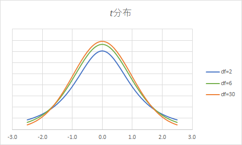
第2の分布のz得点が \[z=\frac{y_i-\overline{y}}{s}\] と計算できるように, 第1の分布のz得点は下のように計算でき, \[z=\frac{y_i-\mu}{\sigma}\] 第3の分布のz得点はこうなります: \[z=\frac{\overline{y}-\mu}{\sigma/\sqrt{n}}\] \(\mu\)の95%の信頼区間を,第3の分布の正規分布の95%の面積(確率)のz得点をもとに推定したいのですが,問題は母分散\(\sigma\)もわからないことなので,ここに\(s\)を代入するt値とその確率分布であるt分布を用いることにします。 t分布は自由度(\(n-1\)) によって形が変わり,自由度が大きくなるほど標準正規分布に近づきます。 \[t=\frac{\overline{y}-\mu}{s/\sqrt{n}}\]
The z scores of the second-type distribution can be calculated as follows:
\[z=\frac{y_i-\overline{y}}{s}\]
The z scores of the first-type distribution can be calculated as follows
\[z=\frac{y_i-\mu}{\sigma}\]
Likewise, the z scores of the third-type distribution can be calculated as follows:
\[z=\frac{\overline{y}-\mu}{\sigma/\sqrt{n}}\]
We want to estimate the 95% confidence interval of \(\mu\) based on the z score of the 95% area (probability) of the standard normal distribution, but the problem is that we do not even know the population variance \(\sigma\), so we will use here the t values which uses \(s\) for \(\sigma\) and its probability distribution of t values, i.e., the t distribution .
The t distribution changes its shape depending on the degrees of freedom n - 1, and the larger the degrees of freedom, the closer it approaches the standard normal distribution.
t distribution
動画で簡単に説明していますが,母平均\(\mu\)の信頼区間は次のように表されます。 \[\overline{y}-t×s/\sqrt{n} ≦ \mu ≦ \overline{y}+t×s/\sqrt{n}\]
As briefly explained in the video, confidence interval of the population mean \(\mu\) is expressed as follows: \[\overline{y}-t×s/\sqrt{n} ≦ \mu ≦ \overline{y}+t×s/\sqrt{n}\]
Video with English subtitles
10.2.5 平均の差と信頼区間/Difference of Means and Confidence Interval
次のような想定です。
上司と雑談が続いていて,上司にはまた新しい疑問が浮かんだようです。
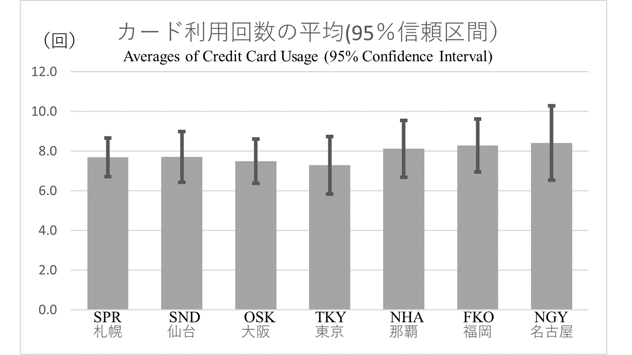
「カードの利用回数って支店ごとに違うのかな?」と上司に問われました。xが支店でyがカード利用回数なら平均の比較だとわかると思います。それでは信頼区間付き棒グラフで比べてみます。
Supposes the following situation. You are still chatting with your boss, and your boss asks another question. "Does the number of card usage differ from branch to branch?" As you know, if x is the branch and y is the number of times the card is used, then the task is comparison of means. Let's compare means by branch in a bar chart with confidence intervals.
動画のように,ピボットテーブルを作ったら平均と標準偏差の値だけコピーして\(n\),\(\sqrt{n}\),\(\frac{s}{\sqrt{n}}×t_{\alpha/2}\)の列を作っておきます。 グラフには使いませんが,確認のためにLCI(信頼区間下限値)とUCI(信頼区間上限値)の列も作ります。
As shown in the video, after creating the pivot table, copy only the mean and standard deviation values and create the columns \(n\), \(\sqrt{n}\), \(\frac{s}{\sqrt{n}}×t_{\alpha/2}\). Although not used in the chart, the LCI (Lower Confidence Interval) and UCI (Upper Confidence Interval) columns are also created for the sake of checking.
棒グラフを作ったら,棒グラフ全体の幅や色を好きにカスタマイズします。そして誤差範囲に\(\frac{s}{\sqrt{n}}×t_{\alpha/2}\)の範囲を指定します。 これで95%信頼区間付き棒グラフが完成です。
After creating the bar chart, customize the width and color of the entire bar chart as you wish. Then, specify an error range of \(\frac{s}{\sqrt{n}}×t_{\alpha/2}\). This completes the bar chart with 95% confidence interval.
Video with English subtitles
Windows/English
Mac/日本語
10.2.6 Python による記述統計/Descriptive Statistics in Python
本セクションではPythonによる記述統計として,describe()による基本統計量,次セクションではPythonによる統計的検定の例として,t検定を紹介します。それでは下記コード1で,kingaku.csvの基本統計量を表示しましょう。
In this section, we introduce summary statistics by describe() as descriptive statistics in Python, and in the next section, we introduce t-test as an example of statistical tests in Python. Now, let us display the summary statistics of kingaku.csv with the following code-1.
import pandas as pd
df5 = pd.read_csv("/content/drive/My Drive/Colab Notebooks/data/kingaku.csv")
df5.describe()
下記コード2は,payment変数の分散を表示します。
Code-2 below displays the variance of the "payment" variable.
df5["payment"].var()
10.2.7 Python による母平均の差の検定/Testing for the Difference between the Population Means in Python
札幌と仙台でpaymentの母平均に差があると言えるかどうかをt検定で確かめます。t検定の前には,等分散の検定を行います。下記コード3では,Levene検定を実施します。
The t-test is used to check if there is a difference in the population mean of "payment" between SPR and SND. Before conducting t-test, a test of equal variances should be performed. In code-3 below, we perform the Levene test.
import scipy.stats as stats
import pandas as pd
spr_pay = df5[df5["branch"] == "SPR"]["payment"]
snd_pay = df5[df5["branch"] == "SND"]["payment"]
var_result = stats.levene(spr_pay, snd_pay)
print(var_result)

Levene検定の結果を受けて,コード4でスチューデントのt検定を実施します。
According to the result of the Levene test, a Student's t-test is performed with code-4.
t_result = stats.ttest_ind(spr_pay, snd_pay)
print(t_result)