11データアナリティクスと機械学習 / Data Analytics and Machine Learning
【目次/TOC】
- データアナリティクスとBI
Data Analytics and BI - 機械学習,深層学習の簡単な紹介
Brief Introduction to Machine Learning and Deep Learning - 機械学習のタスクの実際
Machine Learning Tasks in Practice
1. データアナリティクスとBI/Data Analytics and BI

本ウェブページは『超入門 はじめてのAI・データサイエンス』第11章に記載されたコードを埋め込んでいます。第4章で使い方を学んだColab上でコードを実行すれば,Pythonによる基本の機械学習タスクを体験できます。書籍の最初のセクションでは,Microsoft社のPower BI,Tableau(タブロー),日本語に強いExploratoryなどのBIツールが,BI(ビジネスインテリジェンス),すなわち,データを分析して意味を引き出し,データドリブンな決定につなげるプロセスで用いられていることに言及していますが,最近では,生成AIを搭載したcopilotなどマルチモーダル機能を持つアプリが,情報収集から分析,報告まで,幅広いタスクの遂行に応用されています。
This webpage corresponds to Session 11 of the English website. You can try the codes embedded in this website on Colab as in Session 04, and experience basic tasks of machine learning in Python. Referred in the first section of Session 11 are BI tools such as Microsoft's Power BI, Tableau, and Exploratory, which is useful in Japanese, are used in Business Intelligence, i.e., the process of analyzing data to extract meaning and lead to data-driven decisions. More recently, applications with multimodal capabilities, such as copilot with generative AI, have been applied to perform a wide range of tasks, from collecting information, doing analysis to producing reports.
2.機械学習,深層学習の簡単な紹介/Brief Introduction to Machine Learning and Deep Learning

AI,機械学習,深層学習の関係について,書籍で簡単に紹介しています。
A brief explanation of the relationship between AI, machine learning, and deep learning is provided in the book.
11.2.1 機械学習のタスクの種類/Types of Machine Learning Tasks
書籍では,基本の機械学習タスクに,回帰,分類,クラスタリングのタスクがあることを紹介しています。
The book introduces the basic machine learning tasks of regression, classification, and clustering.
11.2.2 機械学習のプロセス/Machine Learning Processes
書籍では,ホールドアウト法など機械学習のプロセスに触れています。教師あり機械学習ではデータを学習データとテストデータ,あるいは学習データ,検証データ,テストデータの3つに分けます。学習データで構築したモデルをテストデータに適用してその精度を評価し,データの加工や別モデルの試み,ハイパーパラメータの調整によって,Yの予測力の精度を上げていきます。
The book touches on the machine learning process, including the holdout method. In supervised learning machine learning, data is divided into training data and test data or into three: training data, validation data and test data. Training data is used to buid a model, and test data is used to evaluate the performance of the model. Performance of models are improved by preprocessing the data, chosing other models and tuning hyperparameters.
3. 機械学習のタスクの実際/Machine Learning Tasks in Practice
11.3.1 回帰タスク/Regression Task
線形回帰:単回帰分析/Linear Regression: Single Regression Analysis
ここからがコード1です。まずは回帰タスクです。前回,単回帰分析の例で用いたペンギンのヒレの長さと体重について,ヒレの長さから体重を予測する回帰モデルにしてみましょう。下記コード1で,ライブラリとデータの読み込み,そして欠損値の削除,変数の設定をします。
Let's get started with Code1, first for a regression task. In the previous session, we used the flipper length and body mass for the example of simple regression analysis. Let's make a regression model that predicts body mass from flipper length. Use code-1 to import libraries and data, delete missing values and set variables.
import seaborn as sns
df = sns.load_dataset("penguins")
df2 = df.dropna()
x = df2[["flipper_length_mm"]]
y = df2["body_mass_g"]
下記コード2では,モデル構築用の学習(train)データと評価用のテスト(test)データに分割します。機械学習のライブラリであるscikit-learnのtrain_test_splitを用いてデータを分割します。下記のコードでは学習データとテストデータを7:3に分割しています。そのために引数で,train_size = 0.7, test_size = 0.3を指定しています。random_stateというのは乱数のseedのことで,指定しないとそのたびにデータが変わってしまうので,任意の値(ここでは1)を入れて乱数を固定しています。print関数で分割されたそれぞれのデータの数を確認します。
Running code-2 below will result in splitting the data into training data for model building and test data for evaluation. We will split the data using train_test_split of scikit-learn, a machine learning library. In the code below, training data and test data are split in the 7:3 ratio. The random number state is a random number seed, and if it is not specified, the data will change each time, so an arbitrary value (1 in this case) is used to fix the random number. The print function shows the number of each data.
from sklearn.model_selection import train_test_split
x_train, x_test, y_train, y_test = train_test_split(x, y, train_size = 0.7, test_size = 0.3, random_state = 1)
print("サンプルサイズ x_train", len(x_train))
print("サンプルサイズ x_test", len(x_test))
print("サンプルサイズ y_train", len(y_train))
print("サンプルサイズ y_test", len(y_test))
from sklearn.model_selection import train_test_split
x_train,x_test,y_train,y_test = train_test_split(x,y,train_size = 0.7,test_size = 0.3,random_state = 1)
print('sample size x_train',len(x_train))
print('sample size x_test',len(x_test))
print('sample size y_train',len(y_train))
print('sample size y_test',len(y_test))
下記コード3ではscikit-learnのLinearRegressionを用いて,モデルlrを線形回帰(linear regression)に指定し,X_train, Y_trainでモデルを学習させます。コードの3行目まででモデルが構築できたので,4行目でそのモデル用いてx_testデータからYを予測したものをY_predに格納します。Y_predを表示すればどう予測したかを表示できますがその辺りはスキップして,Y_predが実際の値(正解,つまりY_testの値)からどの程度外れているかを,よく用いられる損失関数であるMSE(平均二乗誤差,mean squared error)で見てみます。MSEは下記の式で表されます。また,ペンギンの体重の分散のどの程度がヒレの長さによって予測することができたかを決定係数R2で評価します。
Code-3 below uses scikit-learn's LinearRegression, specifies the model lr as linear regression and trains the model with X_train and Y_train. Since the model has been built by the third line of code, the fourth line uses the model to predict Y from the x_test data and stores it in Y_pred. You can show how you predicted by displaying Y_pred, but I'll skip that part and go on to check how Y_pred deviates from the correct Y (Y_test) using MSE (mean squared error), a commonly used loss function. In addition, let's evaluate how much of the variance in penguin weight could be predicted by fin length with the coefficient of determination R2.
from sklearn.linear_model import LinearRegression
lr = LinearRegression()
lr.fit(x_train, y_train)
下記コード4で,テストデータにモデルを用いて予測します。
Appliy the model to the test data for prediction using code-4 below.
y_pred = lr.predict(x_test)
下記コード5でモデルを評価します。
Run code-5 below to evaluate the model.
from sklearn.metrics import mean_squared_error
y_train_pred = lr.predict(x_train)
print("学習データのMSE: ", mean_squared_error(y_train, y_train_pred))
print("テストデータのMSE: ", mean_squared_error(y_test, y_pred))
from sklearn.metrics import mean_squared_error
y_train_pred = lr.predict(x_train)
print("MSE of training data: ",mean_squared_error(y_train,y_train_pred))
print("MSE of test data: ",mean_squared_error(y_test,y_pred))
下記コード6で決定係数を表示します。
Running code-6 below will result in displaying the coefficient of determination.
from sklearn.metrics import r2_score
print("学習データの決定係数: ", r2_score(y_train, y_train_pred))
print("テストデータの決定係数: ", r2_score(y_test, y_pred))
from sklearn.metrics import r2_score
print("Coefficient of determination of training data: ",r2_score(y_train,y_train_pred))
print("Coefficient of determination of test data: ", r2_score(y_test,y_pred))
重回帰分析/Multiple Regression Analysis
量的データの3つの特徴量から,ターゲットであるペンギンの体重を予測します。下記コード7で,量的データだけのdf2を作ります。
Predict the target data, the body mass of penguins, based on features, the other three quantitative data. Creates df2 with only quantitative data using code-7 below.
features = ["flipper_length_mm", "bill_length_mm", "bill_depth_mm"]
x = df2[features]
y = df2["body_mass_g"].values
ちなみに,書籍の誤植のとおり,targetという変数を作った場合が下記のコード8です。コード7でも8でも変わりません。
By the way, the following code-8 is for the case where the variable "target" is created as in the book. Code-7 or 8 makes no difference.
features = ["flipper_length_mm", "bill_length_mm", "bill_depth_mm"]
target = ["body_mass_g"]
x = df2[features]
y = df2[target]
コード9でデータを分割します。
Run code-9 to split the data.
from sklearn.model_selection import train_test_split
x_train, x_test, y_train, y_test = train_test_split(x, y, test_size = 0.3, random_state= 1)
下記コード10でデータを標準化します。
Use code-10 below to standardize the data.
import pandas as pd
from sklearn.preprocessing import StandardScaler
scaler = StandardScaler()
scaler.fit(x_train)
x_train_std = scaler.transform(x_train)
x_train_std = pd.DataFrame(x_train_std, columns = features)
x_test_std = scaler.transform(x_test)
x_test_std = pd.DataFrame(x_test_std, columns = features)
コード11で学習させます。
The model is trained with code-11.
lr = LinearRegression()
lr.fit(x_train_std, y_train)
コード12で評価します。
Run code-12 to evaluate the model.
y_pred = lr.predict(x_test_std)
y_train_pred = lr.predict(x_train_std)
from sklearn.metrics import mean_squared_error
print("学習データのMSE: ", mean_squared_error(y_train, y_train_pred))
print("テストデータのMSE: ", mean_squared_error(y_test, y_pred))
y_pred = lr.predict(x_test)
y_train_pred = lr.predict(x_train_std)
from sklearn.metrics import mean_squared_error
print("MSE of train data:", mean_squared_error(y_train, y_train_pred))
print("MSE of test data:", mean_squared_error(y_test, y_pred))
コード13で決定係数を確認します。
Use code-13 below to display the coefficient of determination.
from sklearn.metrics import r2_score
print("学習データの決定係数: ", r2_score(y_train, y_train_pred))
print("テストデータの決定係数: ", r2_score(y_test, y_pred))
from sklearn.metrics import r2_score
print("Coefficient of Determination of Learning Data: ", r2_score(y_train,y_train_pred))
print("Coefficient of Determination of Test Data: ", r2_score(y_test,y_pred))
その他の回帰タスクアルゴリズム/Other Regression Task Algorithm
下記コード14はLassoの回帰タスクです。
Code-14 below is for a regression task with Lasso.
from sklearn.linear_model import Lasso
lr2 = Lasso().fit(x_train_std, y_train)
y_pred2 = lr2.predict(x_test_std)
y_train_pred2 = lr.predict(x_train_std)
print("学習データのMSE: ", mean_squared_error(y_train, y_train_pred2))
print("テストデータのMSE: ", mean_squared_error(y_test, y_pred2))
print("学習データの決定係数: ", r2_score(y_train, y_train_pred2))
print("テストデータの決定係数: ", r2_score(y_test, y_pred2))
from sklearn.linear_model import Lasso
lr2 = Lasso().fit(x_train_std, y_train)
y_pred2 = lr2.predict(x_test_std)
y_train_pred2 = lr.predict(x_train_std)
print("MSE of Train Data: ", mean_squared_error(y_train, y_train_pred2))
print("MSE of Test Data: ", mean_squared_error(y_test, y_pred2))
print("Coefficient of Determination of Train Data: ", r2_score(y_train, y_train_pred2))
print("Coefficient of Determination of Test Data: ", r2_score(y_test, y_pred2))
コード15は決定木を用いています。
Code-15 uses decision tree.
from sklearn.tree import DecisionTreeRegressor
from sklearn.tree import export_text
dtr = DecisionTreeRegressor().fit(x_train_std, y_train)
print(export_text(dtr))
下記コード16ではランダムフォレストを用います。
Code-16 below uses random forest.
from sklearn.ensemble import RandomForestRegressor
rfr = RandomForestRegressor().fit(x_train_std, y_train)
y_pred4 = rfr.predict(x_test_std)
y_train_pred4 = rfr.predict(x_train_std)
print("学習データのMSE: ", mean_squared_error(y_train, y_train_pred4))
print("テストデータのMSE: ", mean_squared_error(y_test, y_pred4))
print("学習データの決定係数: ", r2_score(y_train, y_train_pred4))
print("テストデータの決定係数: ", r2_score(y_test, y_pred4))
from sklearn.ensemble import RandomForestRegressor
rfr = RandomForestRegressor().fit(x_train_std, y_train)
y_pred4 = rfr.predict(x_test_std)
y_train_pred4 = rfr.predict(x_train_std)
print("MSE of Train Data: ", mean_squared_error(y_train, y_train_pred4))
print("MSE of Test Data: ", mean_squared_error(y_test, y_pred4))
print("Coefficient of Determination of Train Data: ", r2_score(y_train, y_train_pred4))
print("Coefficient of Determination of Test Data: ", r2_score(y_test, y_pred4))
下記コード17で,勾配ブースティングを用いています。
In code-17 below, gradient boosting is employed.
from sklearn.ensemble import GradientBoostingRegressor
gbr = GradientBoostingRegressor().fit(x_train_std, y_train)
y_pred5 = gbr.predict(x_test_std)
y_train_pred5 = gbr.predict(x_train_std)
print("学習データのMSE: ", mean_squared_error(y_train, y_train_pred5))
print("テストデータのMSE: ", mean_squared_error(y_test, y_pred5))
print("学習データの決定係数: ", r2_score(y_train, y_train_pred5))
print("テストデータの決定係数: ", r2_score(y_test, y_pred5))
from sklearn.ensemble import GradientBoostingRegressor
gbr = GradientBoostingRegressor().fit(x_train_std, y_train)
y_pred5 = gbr.predict(x_test_std)
y_train_pred5 = gbr.predict(x_train_std)
print("MSE of Train Data: ", mean_squared_error(y_train, y_train_pred5))
print("MSE of Test Data: ", mean_squared_error(y_test, y_pred5))
print("Coefficient of Determination of Train Data: ", r2_score(y_train, y_train_pred5))
print("Coefficient of Determination of Test Data: ", r2_score(y_test, y_pred5))
データの前処理とパラメータの調整/Data Preprocessing and Tuning Hyperparameters
下記コード18で,質的データを分析に入れる準備をします。
Code-18 below
prepares qualitative data to be included in the analysis.numeric_features = ["bill_length_mm", "bill_depth_mm", "flipper_length_mm"]
categorical_features = ["species", "island", "sex"]
df2 = df2.replace({"species": {"Adelie": 1, "Chinstrap": 2, "Gentoo": 3}})
df2 = df2.replace({"island": {"Torgersen": 1, "Dream": 2, "Biscoe": 3}})
df2 = df2.replace({"sex": {"Male": 0, "Female": 1}})
df2.head()
コード19でデータを分割します。引用符の中に%dを用いると、その後で定義されている% (X_train.shape[0], X_test.shape[0]))の値を文字列として挿入することができます。\nは改行です。
Run code-19 below to split the data. Using %d within quotation marks, the value of % (X_train.shape[0], X_test.shape[0])) defined afterwards can be inserted as a string. \n makes a newline.
X, Y = df2[["species","island","bill_length_mm", "bill_depth_mm", "flipper_length_mm","sex"]].values, df2["body_mass_g"].values
X_train, X_test, Y_train, Y_test = train_test_split(X, Y, test_size=0.3, random_state=1)
print("学習データ: %d rows\n テストデータ: %d rows" % (X_train.shape[0], X_test.shape[0]))
X, Y = df2[["species","island","bill_length_mm", "bill_depth_mm", "flipper_length_mm","sex"]].values, df2["body_mass_g"].values
X_train, X_test, Y_train, Y_test = train_test_split(X, Y, test_size=0.3, random_state=1)
print("train data: %d rows\n test data: %d rows" % (X_train.shape[0], X_test.shape[0]))
コード20でライブラリを読み込みます。
Import libraries with code-20.
from sklearn.compose import ColumnTransformer
from sklearn.pipeline import Pipeline
from sklearn.impute import SimpleImputer
from sklearn.preprocessing import StandardScaler, OneHotEncoder
from sklearn.linear_model import LinearRegression
import numpy as np
下記コード21でデータの前処理を行います。
Perform data preprocessing using code-21 below.
numeric_features = [2,3,4]
numeric_transformer = Pipeline(steps=[
    ("scaler", StandardScaler())])
categorical_features = [0,1,5]
categorical_transformer = Pipeline(steps=[
    ("onehot", OneHotEncoder(handle_unknown="ignore"))])
preprocessor = ColumnTransformer(
    transformers=[
        ("num", numeric_transformer, numeric_features),
        ("cat", categorical_transformer, categorical_features)])
コード22でハイパーパラメータの調整をします。
Tuning of hyperparameters is conducted with code-22.
from sklearn.ensemble import GradientBoostingRegressor
from sklearn.model_selection import GridSearchCV
from sklearn.metrics import make_scorer, r2_score

alg = GradientBoostingRegressor()

params = {
 "learning_rate": [0.1, 0.5, 1.0],
 "n_estimators" : [50, 100, 150]
 }

score = make_scorer(r2_score)
gridsearch = GridSearchCV(alg, params, scoring=score, cv=3,
return_train_score=True)
gridsearch.fit(X_train, Y_train)
print("最適パラメータの組み合わせ: ", gridsearch.best_params_, "\n")
from sklearn.ensemble import GradientBoostingRegressor
from sklearn.model_selection import GridSearchCV
from sklearn.metrics import make_scorer, r2_score

alg = GradientBoostingRegressor()

params = {
 "learning_rate": [0.1, 0.5, 1.0],
 "n_estimators" : [50, 100, 150]
 }

score = make_scorer(r2_score)
gridsearch = GridSearchCV(alg, params, scoring=score, cv=3,
return_train_score=True)
gridsearch.fit(X_train, Y_train)
print("Bet combination of parameters: ", gridsearch.best_params_, "\n")
コード23で,チューニング後のモデルに前処理したデータを引き渡して回帰タスクを実施します。
In code-23, the regression task is performed by handing over the preprocessed data to the tuned model.
pipeline = Pipeline(steps=[('preprocessor', preprocessor), ('regressor',
                GradientBoostingRegressor(n_estimators=50, learning_rate=0.1))])
best_gbr = pipeline.fit(X_train, (Y_train))

Y_pred7 = best_gbr.predict(X_test)
mse = mean_squared_error(Y_test, Y_pred7)
print("MSE:", mse)
r2 = r2_score(Y_test, Y_pred7)
print("R2 of test data: ", r2)
11.3.2 クラスタリングタスク/Clustering Tasks
k平均法を用いるのに,必要なライブラリをコード24で読み込みます。
In order to use the k-means method, import the necessary libraries code-24.
import numpy as np
import matplotlib.pyplot as plt
!pip install japanize-matplotlib
import japanize_matplotlib
import seaborn as sns
from sklearn.cluster import KMeans
from sklearn.decomposition import PCA
コード25では,lambdaを使って量的データを標準化しています。
Code-25 uses lambda to standardize quantitative data.
df = sns.load_dataset("penguins")
df2 = df.dropna()
features = df2.iloc[:, 2:6].apply(lambda x: (x-x.mean())/x.std(), axis=0)

下記コード26では,主成分分析(第9章参照)を実施して,2つの軸に次元削減をします。
Running code-26 below conducts a principal component analysis (see Session 09) to perform dimensionality reduction to two axes.
pca = PCA(n_components=2).fit(features)
features_2d = pca.transform(features)
コード27で,scikit-learnのk平均法を実施します。
Use code-27 below to conduct the k-means method of scikit-learn.
km = KMeans(n_clusters=3, init="k-means++", n_init=100, max_iter=1000)
km_clusters = km.fit_predict(features.values)
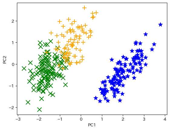
下記コード28でk平均法の結果を可視化します。
Use code-28 below to visualize the result of the k-means method.
def plot_clusters(dim_2, clusters):
    col_dic = {0: "blue", 1: "green", 2:"orange"}
    mrk_dic = {0: "*", 1: "x", 2: "+"}
    colors = [col_dic[x] for x in clusters]
    markers = [mrk_dic[x] for x in clusters]
    for i in range(len(clusters)):
        plt.scatter(dim_2[i][0], dim_2[i][1], color = colors[i],
        marker=markers[i], s=100)
    plt.xlabel("PC1")
    plt.ylabel("PC2")
    plt.show()

plot_clusters(features_2d, km_clusters)
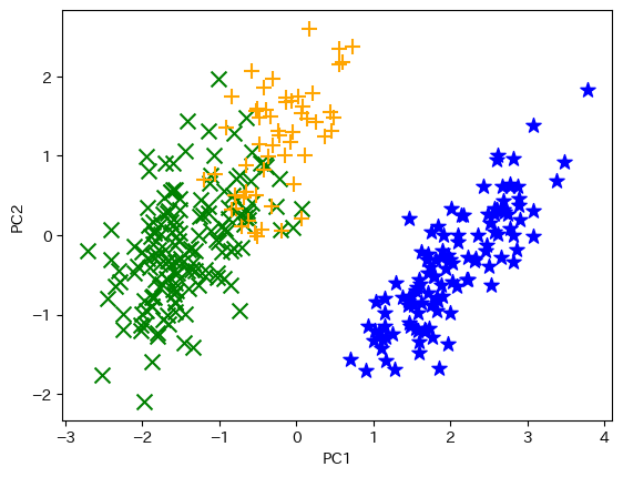
下記コード29では,階層クラスタリングを実施して可視化します。
Running code-29 will result in a hierarchical clustering and its visualization.
from sklearn.cluster import AgglomerativeClustering
agg_model = AgglomerativeClustering(n_clusters=3)
agg_clusters = agg_model.fit_predict(features.values)
plot_clusters(features_2d, agg_clusters)
11.3.3 分類タスク(二値分類)/Classification Task (Binary Classification)
Wisconsin Breast Cancer Datasetを使って診断の特徴量から悪性の乳がんを識別する分類タスクを実施します。コード30でUC Irvineのウェブサイトからデータを取得します。
Perform the classification task of identifying malignant breast cancer from diagnostic features using the Wisconsin Breast Cancer Dataset. Fetch the data from the UC Irvine website with code-30.
!pip install ucimlrepo
from ucimlrepo import fetch_ucirepo
breast_cancer_wisconsin_diagnostic = fetch_ucirepo(id=17)
X = breast_cancer_wisconsin_diagnostic.data.features
Y = breast_cancer_wisconsin_diagnostic.data.targets
pandasを使い,コード31でdf3というデータフレームにしましょう。
With the use of pandas, make it a data frame "df3" with code-31.
df3 = pd.concat([X, Y],axis=1)
df3.head()
データが31列の場合はそのままでよいですが,同じ乳がんデータで33列のデータの場合があります。その場合には,NaNの入った不要な列を削除してください。
If the data has 31 columns, you can leave it as it is, but if your data has 33 columns, delete the unnecessary columns with NaN.
M(悪性)とB(良性)の度数をコード32で確認します。
The frequencies of M (malignant) and B (benign) are identified with code-32.
print("B = ", df3.Diagnosis.str.count("B").sum())
print("M = ", df3.Diagnosis.str.count("M").sum())
コード33で,識別のターゲットであるDiagnosisを0, 1の二値変数にします。識別したいMを1とします。
With code-33, make the target "Diagnosis" a binary variable of 0, 1. Let the target of identification "M" be 1.
df3 = df3.replace({"Diagnosis": {"M": 1, "B": 0}})
df3.info()
コード34で特徴量をx, ターゲットをyとします。
Let x be the feature and y the target with code-34.
x=df3.iloc[:,1:-1].values
y=df3["Diagnosis"].values
コード35でデータを分割します。
Run code-35 to split the data.
from sklearn.model_selection import train_test_split
x_train, x_test, y_train , y_test = train_test_split(x,y,test_size=0.3,
random_state=1)
print ("学習データ: %d\nテストデータ: %d" % (x_train.shape[0], x_test.shape[0]))
from sklearn.model_selection import train_test_split
x_train, x_test, y_train , y_test = train_test_split(x,y,test_size=0.3,
random_state=1)
print ("train data: %d\ntest data: %d" % (x_train.shape[0], x_test.shape[0]))
下記コード36では,モデルを作ってテストデータで予測します。
Use code-36 below to create a model and predict on test data.
from sklearn.linear_model import LogisticRegression
binomial = LogisticRegression(solver="liblinear").fit(x_train, y_train)
y_pred = binomial.predict(x_test)
print("テストデータに対するモデルによる予測: ", y_pred)
print("テストデータの実際の値: ", y_test)
from sklearn.linear_model import LogisticRegression
binomial = LogisticRegression(solver="liblinear").fit(x_train, y_train)
y_pred = binomial.predict(x_test)
print("Model Predictions for Test Data:", y_pred)
print("Actual Values of Test Data: ", y_test)
コード37で混同行列を作ります。
Create confusion matrix with code-37.
from sklearn.metrics import confusion_matrix
cm = confusion_matrix(y_test, y_pred)
print(cm)
コード38で正解率を表示します。
Run code-38 to display accuracy.
from sklearn.metrics import accuracy_score
print("正解率:", accuracy_score(y_test, y_pred))
from sklearn.metrics import accuracy_score
print("Accuracy: ", accuracy_score(y_test, y_pred))
下記コード39では再現率と適合率を表示します。
Use code-39 below to display recall and precision.
from sklearn.metrics import precision_score, recall_score
print("再現率:", recall_score(y_test, y_pred))
print("適合性:", precision_score(y_test, y_pred))
from sklearn.metrics import precision_score, recall_score
print("Recall:", recall_score(y_test, y_pred))
print("Precision:", precision_score(y_test, y_pred))
下記コード40でROC曲線を描きます。
Run code-40 below and display the ROC chart.
from sklearn.metrics import roc_curve
from sklearn.metrics import confusion_matrix
import matplotlib
import matplotlib.pyplot as plt
!pip install japanize-matplotlib
import japanize_matplotlib

y_scores = binomial.predict_proba(x_test)

fpr, tpr, thresholds = roc_curve(y_test, y_scores[:,1])
fig = plt.figure(figsize=(6, 6))
plt.plot([0, 1], [0, 1], "k--")
plt.plot(fpr, tpr)
plt.xlabel("偽陽性率")
plt.ylabel("再現率")
plt.show()
from sklearn.metrics import roc_curve
from sklearn.metrics import confusion_matrix
import matplotlib
import matplotlib.pyplot as plt
!pip install japanize-matplotlib
import japanize_matplotlib

y_scores = binomial.predict_proba(x_test)

fpr, tpr, thresholds = roc_curve(y_test, y_scores[:,1])
fig = plt.figure(figsize=(6, 6))
plt.plot([0, 1], [0, 1], "k--")
plt.plot(fpr, tpr)
plt.xlabel("False Positive Rate")
plt.ylabel("Recall")
plt.show()
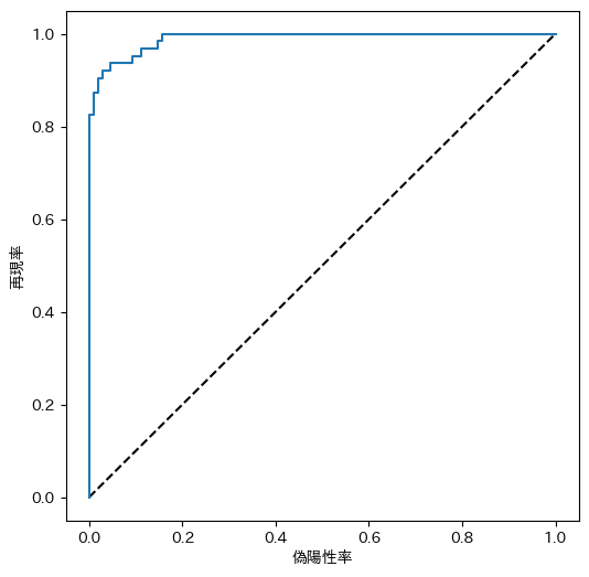
下記コード41では,AUCを算出します。
Running code-41 below will calculate AUC.
from sklearn.metrics import roc_auc_score
auc = roc_auc_score(y_test,y_scores[:,1])
print("AUC: " + str(auc))
11.3.4 分類タスク(多クラス分類)/Classification Task (Multiclass Classification)
コード42では,以下の多クラス分類に必要なライブラリを読み込みます。
Code-42 is to import libraries needed for the following multiclass classification.
import pandas as pd
import numpy as np
import seaborn as sns
from sklearn.impute import SimpleImputer
from sklearn.preprocessing import OrdinalEncoder
from sklearn.pipeline import Pipeline
from sklearn.compose import ColumnTransformer
from sklearn.preprocessing import MinMaxScaler
from sklearn.model_selection import train_test_split
from sklearn.metrics import confusion_matrix
from sklearn.neighbors import KNeighborsClassifier
コード43では,ペンギンデータを読み込みます。
Code-43 is to import penguins dataset.
df = sns.load_dataset("penguins")
df2 = df.dropna()
コード44では,データの分割まで実施します。
All you need to perform up to data splitting is done by running code-44.
x = ["bill_length_mm","bill_depth_mm","flipper_length_mm","body_mass_g"]
y = "species"
x, y = df2[x].values, df2[y].values

x_train, x_test, y_train, y_test = train_test_split(x, y, test_size=0.30,
random_state=1, stratify=y)

print("サンプルサイズ x_train", len(x_train))
print("サンプルサイズ x_test", len(x_test))
print("サンプルサイズ y_train", len(y_train))
print("サンプルサイズ y_test", len(y_test))
x = ["bill_length_mm","bill_depth_mm","flipper_length_mm","body_mass_g"]
y = "species"
x, y = df2[x].values, df2[y].values

x_train, x_test, y_train, y_test = train_test_split(x, y, test_size=0.30,
random_state=1, stratify=y)

print("Sample Size x_train", len(x_train))
print("Sample Size x_test", len(x_test))
print("Sample Size y_train", len(y_train))
print("Sample Size y_test", len(y_test))
コード45で,モデルを構築します。
Build the model with Code-45.
from sklearn.linear_model import LogisticRegression

reg = 0.1

multi_model = LogisticRegression(C=1/reg, solver="lbfgs", multi_class="auto",
max_iter=10000).fit(x_train, y_train)
y_pred = multi_model.predict(x_test)
コード46で,モデルを評価します。
Run code-46 to evaluate the model.
from sklearn.metrics import accuracy_score, precision_score, recall_score

print("正解率:",accuracy_score(y_test, y_pred))
print("適合性:",precision_score(y_test, y_pred, average="macro"))
print("再現率:",recall_score(y_test, y_pred, average="macro"))
from sklearn.metrics import accuracy_score, precision_score, recall_score

print("Accuracy:",accuracy_score(y_test, y_pred))
print("Precision:",precision_score(y_test, y_pred, average="macro"))
print("Recall:",recall_score(y_test, y_pred, average="macro"))
コード47で,混同行列を確認します。
Run code-47 and display the confusion matrix.
from sklearn.metrics import confusion_matrix

mcm = confusion_matrix(y_test, y_pred)
print(mcm)
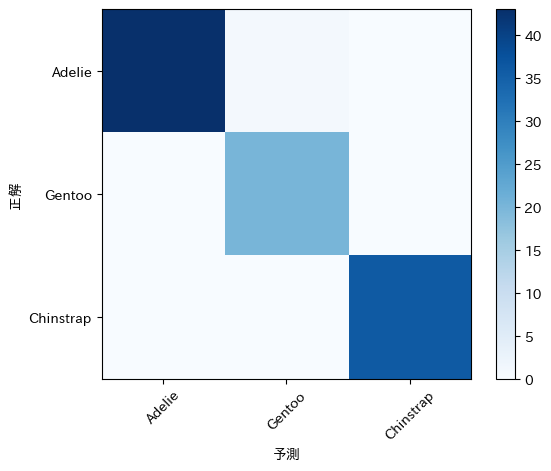
コード48で,ヒートマップを表示します。
Run code-48 to display the heatmap.
import numpy as np
import matplotlib.pyplot as plt
%matplotlib inline

species_classes = ["Adelie", "Gentoo", "Chinstrap"]

plt.imshow(mcm, interpolation="nearest", cmap=plt.cm.Blues)
plt.colorbar()
tick_marks = np.arange(len(species_classes))
plt.xticks(tick_marks, species_classes, rotation=45)
plt.yticks(tick_marks, species_classes)
plt.xlabel("予測")
plt.ylabel("正解")
plt.show()
import numpy as np
import matplotlib.pyplot as plt
%matplotlib inline

species_classes = ["Adelie", "Gentoo", "Chinstrap"]

plt.imshow(mcm, interpolation="nearest", cmap=plt.cm.Blues)
plt.colorbar()
tick_marks = np.arange(len(species_classes))
plt.xticks(tick_marks, species_classes, rotation=45)
plt.yticks(tick_marks, species_classes)
plt.xlabel("Prediction")
plt.ylabel("Label")
plt.show()