12.1 画像認識の機械学習

本ウェブページは『超入門 はじめてのAI・データサイエンス』第12章に記載されたコードを埋め込んでいます。第4章で使い方を学んだColab上でコードを実行すれば,基本の画像認識教材として使われるMNISTを体験できます。
12.1.1 手書き数字データセット「MNIST」
ここで使用するMNISTとは,Mixed National Institute of Standards and Technology databaseの略で,手書き数字のデータセットです。
12.1.2 MNIST データセットの読み込みとデータの成形
書籍の指示通りGPUを選択したら,早速下記のコード1でMNISTデータセットを読み込みます。
コード 1
from tensorflow.keras.datasets import mnist
(x_train, y_train), (x_test, y_test) = mnist.load_data()下記コード2で,データの前処理をします。
コード 2
x_train = x_train.reshape(-1, 28, 28, 1) / 255.0
x_test = x_test.reshape(-1, 28, 28, 1) / 255.0下記コード3で,ラベルデータの前処理をします。
コード 3
import tensorflow as tf
y_train = tf.keras.utils.to_categorical(y_train, num_classes = 10)
y_test = tf.keras.utils.to_categorical(y_test, num_classes = 10)
12.1.3 機械学習モデルの構築
下記コード4で,モデルを作成します。
コード 4
# 必要なモジュールを読み込む
# importing necessary modules
from tensorflow.keras.models import Sequential
from tensorflow.keras.layers import Conv2D, MaxPooling2D, Flatten, Dense, Dropout

# kerasでモデルを積み重ねる土台を呼び出す
# calling the foundation for stacking models with keras
model = Sequential()

# 畳み込みフィルターを設定する
# 32 convolution filters used each of size 3x3
model.add(Conv2D(32, kernel_size = (3, 3), activation = "relu",
input_shape = (28, 28, 1)))
# 64 convolution filters used each of size 3x3
model.add(Conv2D(64, (3, 3), activation = "relu"))

# プーリング処理を施す
# choose the best features via pooling
model.add(MaxPooling2D(pool_size = (2, 2)))

# ドロップアウト法を適用する
# randomly turn neurons on and off to improve convergence
model.add(Dropout(0.25))

# Flattenを用いて1次元化する
# flatten since too many dimensions, we only want a classification output
model.add(Flatten())

# 全結合を1次元化されたデータに対して行う
# fully connected to get all relevant data
model.add(Dense(128, activation = "relu"))

# 活性化関数を設定し,予測を確率で返してくれる
# output a softmax to squash the matrix into output probabilities
model.add(Dense(10, activation = "softmax"))コード5で,モデルをコンパイルします。
コード 5
# 最適化関数,損失関数, 評価関数を設定する
# setting optimizer, loss function, and metrics
model.compile(optimizer = "adam",
              loss = "categorical_crossentropy",
              metrics = ["accuracy"])
12.1.4 モデルの学習
下記コード6では,データでモデルを学習させます。
コード 6
model.fit(x_train, y_train, batch_size = 128, epochs = 10,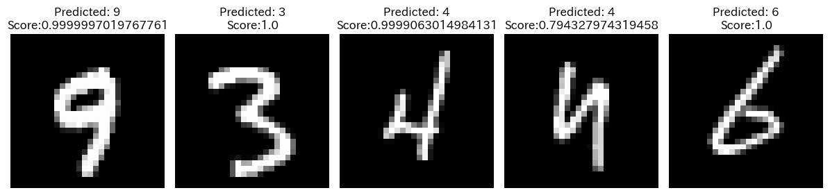
validation_data = (x_test, y_test))下記コード7は,画像とモデルによる判断の確認です。
コード 7
import numpy as np
import matplotlib.pyplot as plt

# テストセットからランダムに画像を抜き出す
# Select a random subset of images from the test set
num_images = 5
np.random.seed(seed = 2)
random_indices = np.random.randint(0, len(x_test), num_images)
images = x_test[random_indices]
labels = y_test[random_indices]

# 選択した画像について予測する
# Make predictions on the selected images
predictions = model.predict(images)
predicted_labels = np.argmax(predictions, axis = 1)

# 画像と予測されたラベルおよびスコアを表示する
# Display the images with their predicted labels and scores
fig, axes = plt.subplots(1, num_images, figsize = (12, 3))

for i in range(num_images):
    axes[i].imshow(images[i].reshape(28, 28), cmap = "gray")
    axes[i].axis("off")
    axes[i].set_title(
        f"Predicted: {predicted_labels[i]}\nScore:{round(np.max(predictions[i]), 8)}"
        )

plt.tight_layout()
plt.show()