超入門はじめてのAI・データサイエンス

11.3 機械学習のタスクの実際

11.3.1 回帰タスク

線形回帰：単回帰分析

ここからが実習パートになります。まずは回帰タスクです。前回，単回帰分析の例で用いたペンギンのヒレの長さと体重について，ヒレの長さから体重を予測する回帰モデルにしてみましょう。下記コード1で，ライブラリとデータの読み込み，そして欠損値の削除，変数の設定をします。

コード 1

import seaborn as sns
df = sns.load_dataset("penguins")
df2 = df.dropna()
x = df2[["flipper_length_mm"]]
y = df2["body_mass_g"]

モデル構築用の学習（train）データと評価用のテスト（test）データに分割します。機械学習のライブラリであるscikit-learnのtrain_test_splitを用いてデータを分割します。

下記のコード2では学習データとテストデータを7:3に分割しています。そのために引数で，train_size = 0.7, test_size = 0.3を指定しています。random_stateというのは乱数のseedのことで，指定しないとそのたびにデータが変わってしまうので，任意の値（ここでは1）を入れて乱数を固定しています。print関数で分割されたそれぞれのデータの数を確認します。

コード 2

from sklearn.model_selection import train_test_split
x_train, x_test, y_train, y_test = train_test_split(x, y, train_size = 0.7, test_size = 0.3, random_state = 1)
print("サンプルサイズ x_train", len(x_train))
print("サンプルサイズ x_test", len(x_test))
print("サンプルサイズ y_train", len(y_train))
print("サンプルサイズ y_test", len(y_test))

下記コード3では，scikit-learnのLinearRegressionを用いて，モデルlrを線形回帰（linear regression）に指定し，X_train, Y_trainでモデルを学習させます。

コードの3行目まででモデルが構築できたので，4行目でそのモデル用いてx_testデータからYを予測したものをY_predに格納します。Y_predを表示すればどう予測したかを表示できますが，その辺りはスキップして，Y_predが実際の値（正解，つまりY_testの値）からどの程度外れているかを，よく用いられる損失関数であるMSE（平均二乗誤差，mean squared error）で見てみます。また，ペンギンの体重の分散のどの程度がヒレの長さによって予測することができたかを決定係数で評価します。

コード 3

from sklearn.linear_model import LinearRegression
lr = LinearRegression()
lr.fit(x_train, y_train)

下記コード4で，テストデータにモデルを用いて予測します。

コード 4

y_pred = lr.predict(x_test)

下記コード5で，モデルを評価します。

コード 5

from sklearn.metrics import mean_squared_error
y_train_pred = lr.predict(x_train)
print("学習データのMSE: ", mean_squared_error(y_train, y_train_pred)) 
print("テストデータのMSE: ", mean_squared_error(y_test, y_pred))

下記コード6で，決定係数を表示します。

コード 6

from sklearn.metrics import r2_score
print("学習データの決定係数: ", r2_score(y_train, y_train_pred))
print("テストデータの決定係数: ", r2_score(y_test, y_pred))

重回帰分析

量的データの3つの特徴量から，ターゲットであるペンギンの体重を予測します。下記コード7で，量的データだけのdf2を作ります。

コード 7

features = ["flipper_length_mm", "bill_length_mm", "bill_depth_mm"]
x = df2[features]
y = df2["body_mass_g"].values

ちなみに，書籍の誤植のとおり，targetという変数を作った場合が下記のコード8です。コード7でも8でも変わりません。

コード 8

features = ["flipper_length_mm", "bill_length_mm", "bill_depth_mm"]
target = ["body_mass_g"]
x = df2[features]
y = df2[target]

コード9でデータを分割します。

コード 9

from sklearn.model_selection import train_test_split
x_train, x_test, y_train, y_test = train_test_split(x, y, test_size = 0.3, random_state = 1)

下記コード10でデータを標準化します。

コード 10

import pandas as pd
from sklearn.preprocessing import StandardScaler
scaler = StandardScaler()
scaler.fit(x_train)
x_train_std = scaler.transform(x_train)
x_train_std = pd.DataFrame(x_train_std, columns = features)
x_test_std = scaler.transform(x_test)
x_test_std = pd.DataFrame(x_test_std, columns = features)

コード11で学習させます。

コード 11

lr = LinearRegression()
lr.fit(x_train_std, y_train)

下記コード12で評価します。

コード 12

y_pred = lr.predict(x_test_std)
y_train_pred = lr.predict(x_train_std)
from sklearn.metrics import mean_squared_error
print("学習データのMSE: ", mean_squared_error(y_train, y_train_pred)) 
print("テストデータのMSE: ", mean_squared_error(y_test, y_pred))

下記コード13で決定係数を確認します。

コード 13

from sklearn.metrics import r2_score
print("学習データの決定係数: ", r2_score(y_train, y_train_pred))
print("テストデータの決定係数: ", r2_score(y_test, y_pred))

その他の回帰タスクアルゴリズム

下記コード14は，Lassoの回帰タスクです。

コード 14

from sklearn.linear_model import Lasso
lr2 = Lasso().fit(x_train_std, y_train)
y_pred2 = lr2.predict(x_test_std)
y_train_pred2 = lr.predict(x_train_std)
print("学習データのMSE: ", mean_squared_error(y_train, y_train_pred2))
print("テストデータのMSE: ", mean_squared_error(y_test, y_pred2))
print("学習データの決定係数: ", r2_score(y_train, y_train_pred2))
print("テストデータの決定係数: ", r2_score(y_test, y_pred2))

コード15は決定木を用いています。

コード 15

from sklearn.tree import DecisionTreeRegressor
from sklearn.tree import export_text
dtr = DecisionTreeRegressor().fit(x_train_std, y_train)
print(export_text(dtr))

下記コード16ではランダムフォレストを用います。

コード 16

from sklearn.ensemble import RandomForestRegressor
rfr = RandomForestRegressor().fit(x_train_std, y_train)
y_pred4 = rfr.predict(x_test_std)
y_train_pred4 = rfr.predict(x_train_std)
print("学習データのMSE: ", mean_squared_error(y_train, y_train_pred4))
print("テストデータのMSE: ", mean_squared_error(y_test, y_pred4))
print("学習データの決定係数: ", r2_score(y_train, y_train_pred4))
print("テストデータの決定係数: ", r2_score(y_test, y_pred4))

下記コード17で，勾配ブースティングを用いています。ちなみに勾配ブースティイングの「勾配」は、MSEなどの損失関数の微分を勾配と呼ぶことに由来しています。個別のデータ点における損失関数\(L\)に対する微分 \(\frac{d}{dx}f(x)\) から誤差の方向と大きさがわかるので、誤差が最小になるように繰り返させる方法です。

個別のデータ点における損失関数
\[L=(x-\hat{x})^2 \] 損失関数の勾配（微分）
\[\frac{dL}{d\hat{x}}\]

コード 17

from sklearn.ensemble import GradientBoostingRegressor
gbr = GradientBoostingRegressor().fit(x_train_std, y_train)
y_pred5 = gbr.predict(x_test_std)
y_train_pred5 = gbr.predict(x_train_std)
print("学習データのMSE: ", mean_squared_error(y_train, y_train_pred5))
print("テストデータのMSE: ", mean_squared_error(y_test, y_pred5))
print("学習データの決定係数: ", r2_score(y_train, y_train_pred5))
print("テストデータの決定係数: ", r2_score(y_test, y_pred5))

データの前処理とパラメータの調整

下記コード18で，質的データを分析に入れる準備をします。

コード 18

numeric_features = ["bill_length_mm", "bill_depth_mm", "flipper_length_mm"]
categorical_features = ["species", "island", "sex"]
df2 = df2.replace({"species": {"Adelie": 1, "Chinstrap": 2, "Gentoo": 3}})
df2 = df2.replace({"island": {"Torgersen": 1, "Dream": 2, "Biscoe": 3}})
df2 = df2.replace({"sex": {"Male": 0, "Female": 1}})
df2.head()

コード19でデータを分割します。引用符の中に%dを用いると，その後で定義されている% (X_train.shape[0], X_test.shape[0]))の値を文字列として挿入することができます。＼nは改行です。

コード 19

X, Y = df2[["species", "island", "bill_length_mm", "bill_depth_mm", "flipper_length_mm", "sex"]].values, df2["body_mass_g"].values
X_train, X_test, Y_train, Y_test = train_test_split(X, Y, test_size = 0.3, random_state = 1)
print("学習データ: %d rows\n テストデータ: %d rows" % (X_train.shape[0], X_test.shape[0]))

コード20でライブラリを読み込みます。

コード 20

from sklearn.compose import ColumnTransformer
from sklearn.pipeline import Pipeline
from sklearn.impute import SimpleImputer
from sklearn.preprocessing import StandardScaler, OneHotEncoder
from sklearn.linear_model import LinearRegression
import numpy as np

下記コード21で，データの前処理を行います。

コード 21

numeric_features = [2, 3, 4]
numeric_transformer = Pipeline(steps = [
    ("scaler", StandardScaler())])
categorical_features = [0, 1, 5]
categorical_transformer = Pipeline(steps = [
    ("onehot", OneHotEncoder(handle_unknown = "ignore"))])
preprocessor = ColumnTransformer(
    transformers = [
        ("num", numeric_transformer, numeric_features),
        ("cat", categorical_transformer, categorical_features)])

コード22で，ハイパーパラメータの調整をします。

コード 22

from sklearn.ensemble import GradientBoostingRegressor
from sklearn.model_selection import GridSearchCV
from sklearn.metrics import make_scorer, r2_score

alg = GradientBoostingRegressor()

params = {
 "learning_rate": [0.1, 0.5, 1.0],
 "n_estimators" : [50, 100, 150]
 }

score = make_scorer(r2_score)
gridsearch = GridSearchCV(alg, params, scoring = score, cv = 3, 
return_train_score = True)
gridsearch.fit(X_train, Y_train)
print("最適パラメータの組み合わせ: ", gridsearch.best_params_, "\n")

コード23で，チューニング後のモデルに前処理したデータを引き渡して回帰タスクを実施します。

コード 23

pipeline = Pipeline(steps = [('preprocessor', preprocessor), ('regressor',
                GradientBoostingRegressor(n_estimators = 50, learning_rate = 0.1))])
best_gbr = pipeline.fit(X_train, (Y_train))

Y_pred7 = best_gbr.predict(X_test)
mse = mean_squared_error(Y_test, Y_pred7)
print("MSE:", mse)
r2 = r2_score(Y_test, Y_pred7)
print("R2 of test data: ", r2)

11.3.2 クラスタリングタスク

k平均法を用いるのに，必要なライブラリをコード24で読み込みます。

コード 24

import numpy as np
import matplotlib.pyplot as plt
!pip install japanize-matplotlib
import japanize_matplotlib
import seaborn as sns
from sklearn.cluster import KMeans
from sklearn.decomposition import PCA

コード25では，lambdaを使って量的データを標準化しています。

コード 25

df = sns.load_dataset("penguins")
df2 = df.dropna()
features = df2.iloc[:, 2:6].apply(lambda x: (x-x.mean())/x.std(), axis = 0)

下記コード26では，主成分分析（第9章参照）を実施して，2つの軸に次元削減をします。

コード 26

pca = PCA(n_components = 2).fit(features)
features_2d = pca.transform(features)

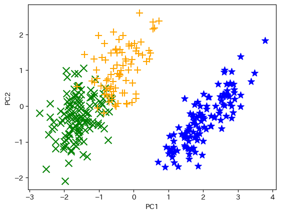
コード27で，scikit-learnのk平均法を実施します。

コード 27

km = KMeans(n_clusters = 3, init = "k-means++", n_init = 100, max_iter = 1000)
km_clusters = km.fit_predict(features.values)

下記コード28で，k平均法の結果を可視化します。

コード 28

def plot_clusters(dim_2, clusters):
    col_dic = {0: "blue", 1: "green", 2:"orange"}
    mrk_dic = {0: "*", 1: "x", 2: "+"}
    colors = [col_dic[x] for x in clusters]
    markers = [mrk_dic[x] for x in clusters]
    for i in range(len(clusters)):
        plt.scatter(dim_2[i][0], dim_2[i][1], color = colors[i], 
        marker = markers[i], s = 100)
    plt.xlabel("PC1")
    plt.ylabel("PC2")
    plt.show()

plot_clusters(features_2d, km_clusters)

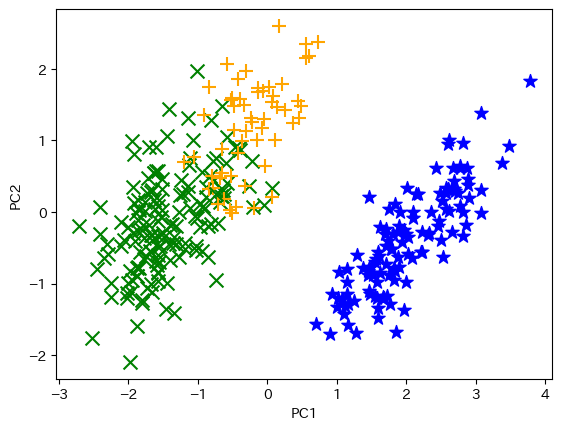
下記コード29では，階層クラスタリングを実施して可視化します。

コード 29

from sklearn.cluster import AgglomerativeClustering
agg_model = AgglomerativeClustering(n_clusters = 3)
agg_clusters = agg_model.fit_predict(features.values)
plot_clusters(features_2d, agg_clusters)

11.3.3 分類タスク(二値分類)

Wisconsin Breast Cancer Datasetを使って診断の特徴量から悪性の乳がんを識別する分類タスクを実施します。コード30でUC Irvineのウェブサイトからデータを取得します。

コード 30

!pip install ucimlrepo
from ucimlrepo import fetch_ucirepo
breast_cancer_wisconsin_diagnostic = fetch_ucirepo(id = 17)
X = breast_cancer_wisconsin_diagnostic.data.features
Y = breast_cancer_wisconsin_diagnostic.data.targets

pandasを使い，コード31でdf3というデータフレームにしましょう。

コード 31

df3 = pd.concat([X, Y],axis = 1)
df3.head()

データが31列の場合はそのままでよいですが，同じ乳がんデータで33列のデータの場合があります。その場合には，NaNの入った不要な列を削除してください。

M（悪性）とB（良性）の度数をコード32で確認します。

コード 32

print("B = ", df3.Diagnosis.str.count("B").sum())
print("M = ", df3.Diagnosis.str.count("M").sum())

コード33で，識別のターゲットであるDiagnosisを0, 1の二値変数にします。識別したいMを1とします。

コード 33

df3 = df3.replace({"Diagnosis": {"M": 1, "B": 0}})
df3.info()

下記コード34で，特徴量をx, ターゲットをyとします。

コード 34

x = df3.iloc[:, 1:-1].values
y = df3["Diagnosis"].values

下記コード35で，データを分割します。

コード 35

from sklearn.model_selection import train_test_split
x_train, x_test, y_train, y_test = train_test_split(x, y, test_size = 0.3,
random_state = 1)
print ("学習データ: %d\nテストデータ: %d" % (x_train.shape[0], x_test.shape[0]))

下記コード36では，モデルを作ってテストデータで予測します。

コード 36

from sklearn.linear_model import LogisticRegression
binomial = LogisticRegression(solver="liblinear").fit(x_train, y_train)
y_pred = binomial.predict(x_test)
print("テストデータに対するモデルによる予測: ", y_pred)
print("テストデータの実際の値: ", y_test)

コード37で，混同行列を作ります。

コード 37

from sklearn.metrics import confusion_matrix
cm = confusion_matrix(y_test, y_pred)
print(cm)

下記コード38で，正解率を表示します。

コード 38

from sklearn.metrics import accuracy_score
print("正解率:", accuracy_score(y_test, y_pred))

下記コード39では，再現率と適合率を表示します。

コード 39

from sklearn.metrics import precision_score, recall_score
print("再現率:", recall_score(y_test, y_pred))
print("適合性:", precision_score(y_test, y_pred))

下記コード40で，ROC曲線を描きます。

コード 40

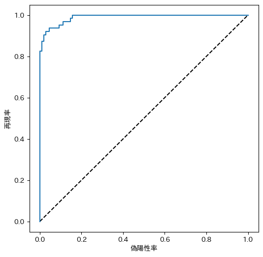
from sklearn.metrics import roc_curve
from sklearn.metrics import confusion_matrix
import matplotlib
import matplotlib.pyplot as plt
!pip install japanize-matplotlib
import japanize_matplotlib

y_scores = binomial.predict_proba(x_test)

fpr, tpr, thresholds = roc_curve(y_test, y_scores[:, 1])
fig = plt.figure(figsize = (6, 6))
plt.plot([0, 1], [0, 1], "k--")
plt.plot(fpr, tpr)
plt.xlabel("偽陽性率")
plt.ylabel("再現率")
plt.show()

下記コード41で，AUCを算出します。

コード 41

from sklearn.metrics import roc_auc_score
auc = roc_auc_score(y_test,y_scores[:, 1])
print("AUC: " + str(auc))

11.3.4 分類タスク(多クラス分類)

コード42では，以下の多クラス分類に必要なライブラリを読み込みます。

コード 42

import pandas as pd
import numpy as np
import seaborn as sns
from sklearn.impute import SimpleImputer
from sklearn.preprocessing import OrdinalEncoder
from sklearn.pipeline import Pipeline
from sklearn.compose import ColumnTransformer
from sklearn.preprocessing import MinMaxScaler
from sklearn.model_selection import train_test_split
from sklearn.metrics import confusion_matrix
from sklearn.neighbors import KNeighborsClassifier

コード43では，ペンギンデータを読み込みます。

コード 43

df = sns.load_dataset("penguins")
df2 = df.dropna()

コード44では，データの分割まで実施します。

コード 44

x = ["bill_length_mm", "bill_depth_mm", "flipper_length_mm", "body_mass_g"] 
y = "species"
x, y = df2[x].values, df2[y].values

x_train, x_test, y_train, y_test = train_test_split(x, y, test_size = 0.30, 
random_state = 1, stratify = y)

print("サンプルサイズ x_train", len(x_train))
print("サンプルサイズ x_test", len(x_test))
print("サンプルサイズ y_train", len(y_train))
print("サンプルサイズ y_test", len(y_test))

コード45で，モデルを構築します。

コード 45

from sklearn.linear_model import LogisticRegression

reg = 0.1

multi_model = LogisticRegression(C = 1/reg, solver = "lbfgs", multi_class = "auto", 
max_iter = 10000).fit(x_train, y_train)
y_pred = multi_model.predict(x_test)

下記コード46で，モデルを評価します。

コード 46

from sklearn.metrics import accuracy_score, precision_score, recall_score

print("正解率:", accuracy_score(y_test, y_pred))
print("適合性:", precision_score(y_test, y_pred, average = "macro"))
print("再現率:", recall_score(y_test, y_pred, average = "macro"))

下記コード47で，混同行列を確認します。

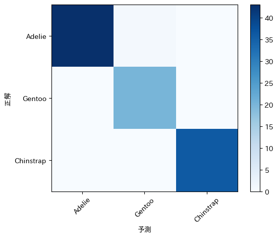
コード 47

from sklearn.metrics import confusion_matrix

mcm = confusion_matrix(y_test, y_pred)
print(mcm)

下記コード48で，ヒートマップを表示します。

コード 48

import numpy as np
import matplotlib.pyplot as plt
%matplotlib inline

species_classes = ["Adelie", "Gentoo", "Chinstrap"]

plt.imshow(mcm, interpolation = "nearest", cmap = plt.cm.Blues)
plt.colorbar()
tick_marks = np.arange(len(species_classes))
plt.xticks(tick_marks, species_classes, rotation = 45)
plt.yticks(tick_marks, species_classes)
plt.xlabel("予測")
plt.ylabel("正解")
plt.show()

About Website

お問合せ先